Combining maps and patterns with {ggplot2}
Visualization
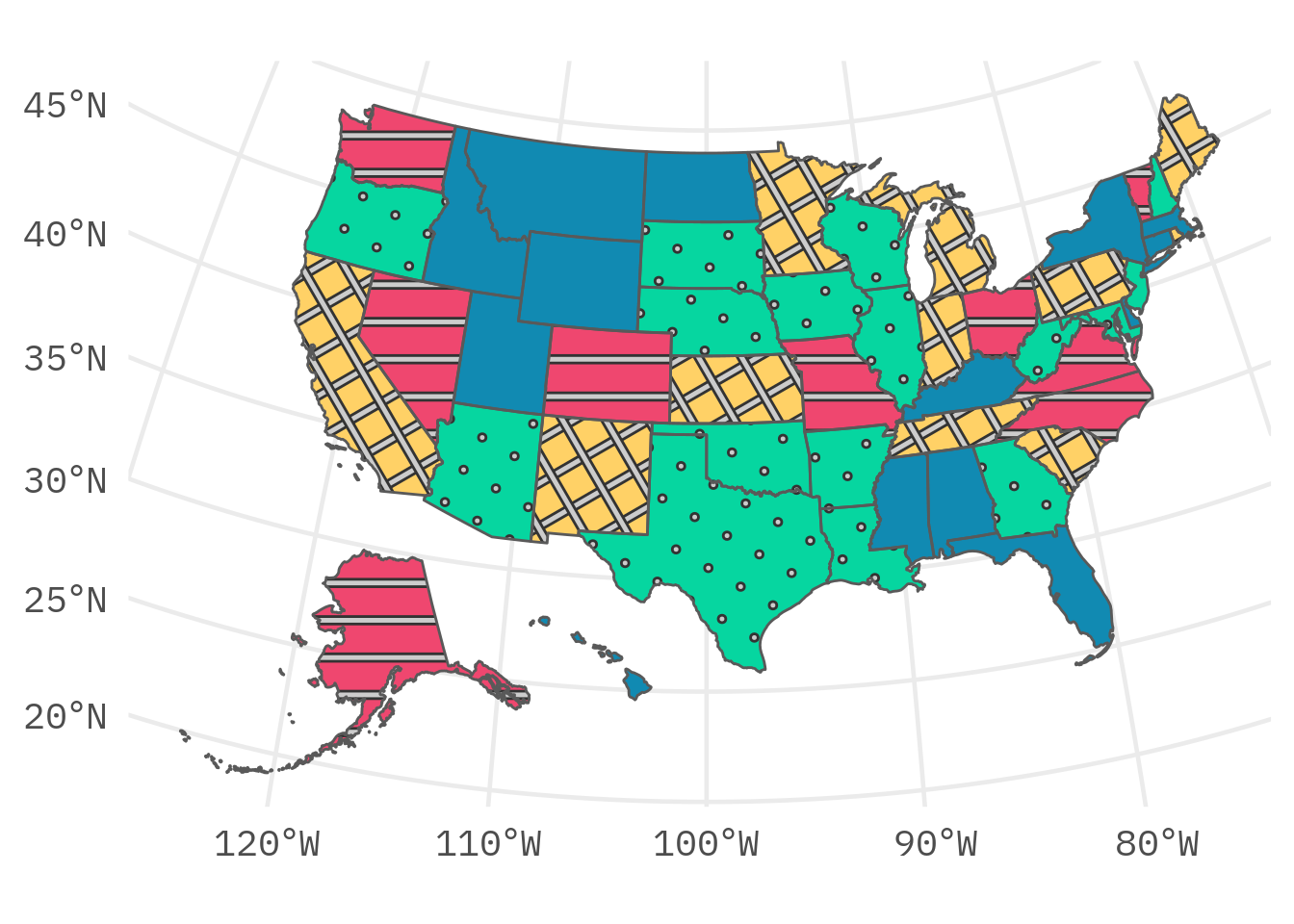
In this video I show you how you can create a map of the US with patterns inside of state borders.
In this post, I will show you how to combine the two cool packages {usmap} and {ggpattern} to create US maps with patterns like this:
And before we dive in, let me tell you that there’s also a video version of this blog post available. You can find it on YouTube:
Get the data
Alright, the first thing that we need to do is to get the data for our US map. We can do that with the {usmap} package. Here’s how this package works. At the core it has two functions: plot_usmap() and us_map(). The first one can - in one line of code - create a US map for you.
library(tidyverse)
library(usmap)
# US States
plot_usmap(regions = 'states')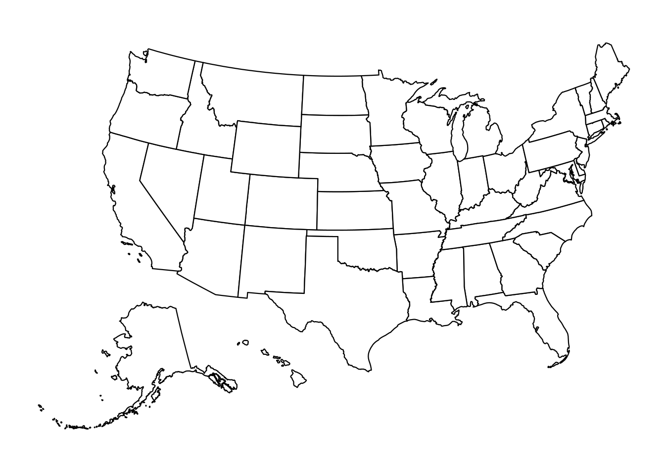
# US Counties
plot_usmap(regions = 'counties')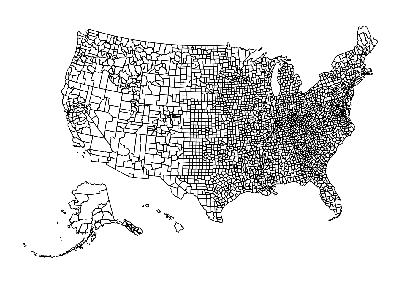
The ease that this function provides is pretty incredible if you ask me. But this function is not what we need here. We want to get the underlying data. That can be done with us_map().
us_map(regions = 'states')
## Simple feature collection with 51 features and 3 fields
## Geometry type: MULTIPOLYGON
## Dimension:     XY
## Bounding box:  xmin: -2590847 ymin: -2608151 xmax: 2523583 ymax: 731405.7
## Projected CRS: NAD27 / US National Atlas Equal Area
## # A tibble: 51 × 4
##    fips  abbr  full                                                         geom
##    <chr> <chr> <chr>                                          <MULTIPOLYGON [m]>
##  1 02    AK    Alaska               (((-2396840 -2547726, -2393291 -2546396, -2…
##  2 01    AL    Alabama              (((1093779 -1378539, 1093270 -1374227, 1092…
##  3 05    AR    Arkansas             (((483066 -927786.9, 506063 -926262.2, 5315…
##  4 04    AZ    Arizona              (((-1388677 -1254586, -1389182 -1251858, -1…
##  5 06    CA    California           (((-1719948 -1090032, -1709613 -1090025, -1…
##  6 08    CO    Colorado             (((-789537.1 -678772.6, -789536.6 -678768.3…
##  7 09    CT    Connecticut          (((2161728 -83727.16, 2177177 -65210.71, 21…
##  8 11    DC    District of Columbia (((1955475 -402047.2, 1960230 -393564, 1964…
##  9 10    DE    Delaware             (((2042501 -284358, 2043073 -279990.9, 2044…
## 10 12    FL    Florida              (((1855614 -2064805, 1860160 -2054368, 1867…
## # ℹ 41 more rows
This function returns a so-called simple feature collection with the geometry of the US states in the geom column of a tibble. For the purpose of this blog post, you can treat this object like any other tibble. And if your output looks a little bit different and gives you just a very long data.frame, then you may have to update your {usmap} package or even use the dev-version via:
devtools::install_github("pdil/usmap")Plot the data
The really cool thing about our data set is that it works perfectly with the geom_sf() layer. You can just pass the data to ggplot and use geom_sf(). See:
us_map(regions = 'states') |>
  ggplot() +
  geom_sf() +
  theme_minimal(base_size = 18, base_family = 'IBM Plex Mono')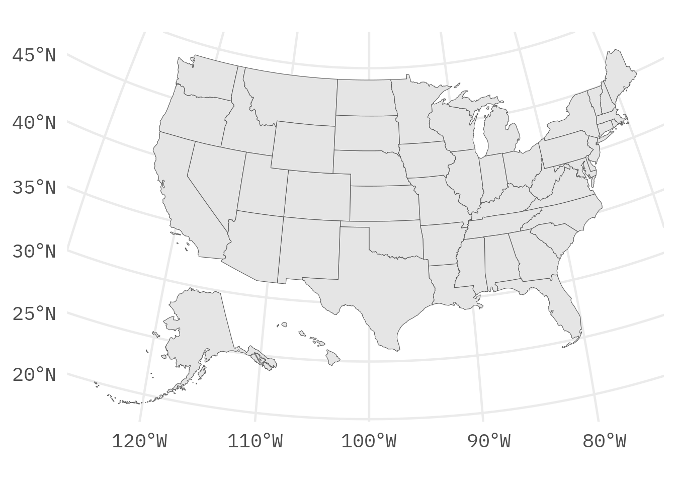
Neat how that works, isn’t it? The geom_sf() layer automatically picks out the geom column and does its thing. And since this is a ggplot, we can do all the usual things. Like map the fill color to a variable in our data set. Here, let’s use the full column as it corresponds to the full name of a state.
us_map(regions = 'states') |>
  ggplot() +
  geom_sf(aes(fill = full)) +
  theme_minimal(base_size = 18, base_family = 'IBM Plex Mono')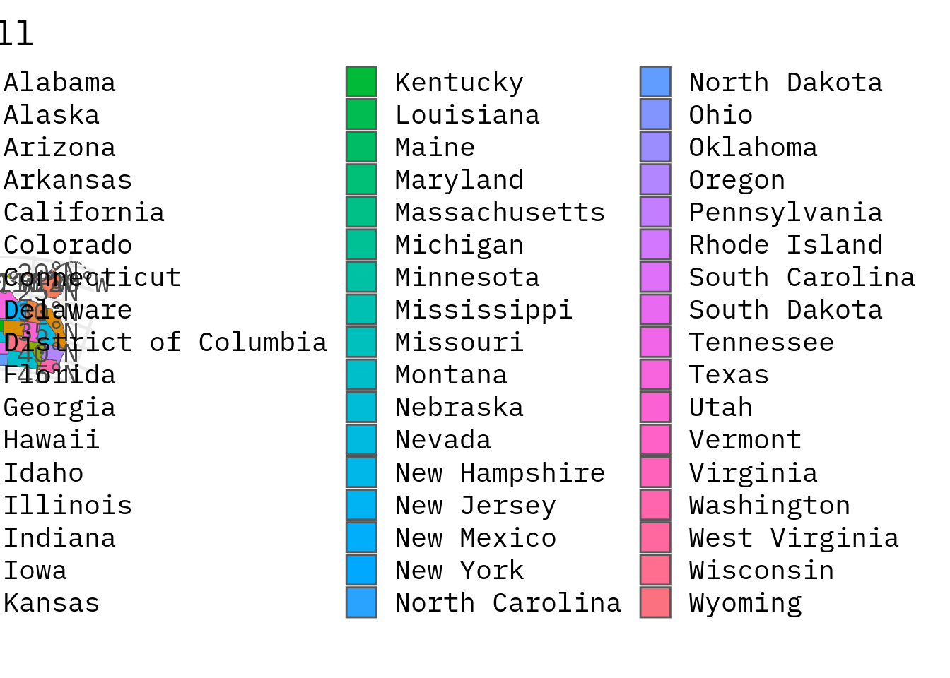
That’s a lot of colors. So let’s remove the legend. This is normally not a good strategy to deal with too many colors. But for this blog post it’s okay.
us_map(regions = 'states') |>
  ggplot() +
  geom_sf(aes(fill = full)) +
  theme_minimal(base_size = 18, base_family = 'IBM Plex Mono') +
  theme(legend.position = 'none')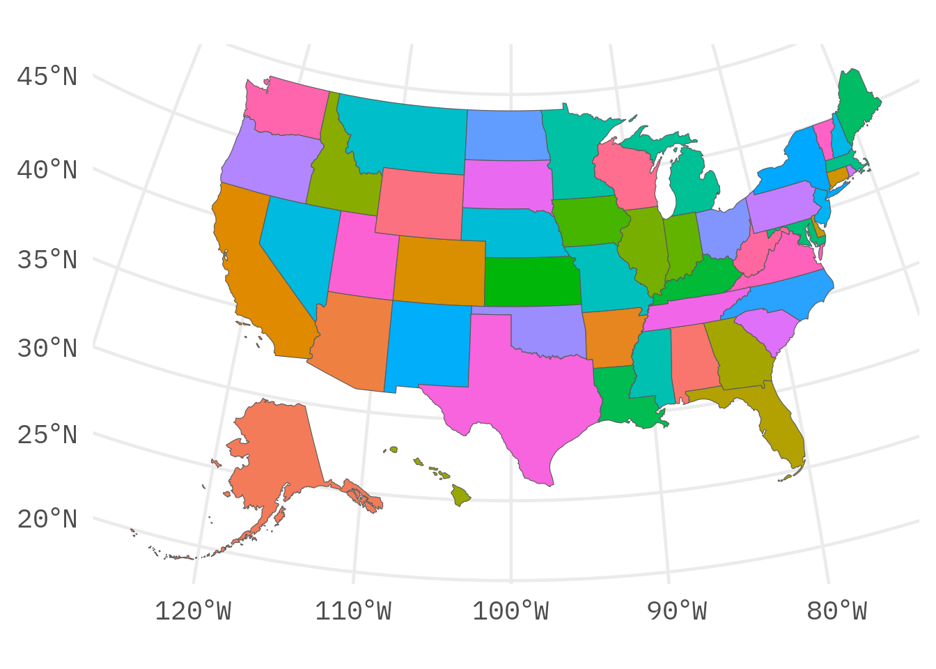
Sidenote: If you’re looking for map-related content, I have a video where I build an elaborate chart that uses a lot of maps of the US. You can find the video here:
Group the data
So now that we know how the geom_sf() layer works, let us group our states. These groups will then be colored differently. And we’ll add patterns to the groups too.
set.seed(2522)
grouped_data <- us_map() |>
  mutate(
    group = sample(
      c('A', 'B', 'C', 'D'),
      size = 51,
      replace = TRUE
    )
  )
grouped_data
## Simple feature collection with 51 features and 4 fields
## Geometry type: MULTIPOLYGON
## Dimension:     XY
## Bounding box:  xmin: -2590847 ymin: -2608151 xmax: 2523583 ymax: 731405.7
## Projected CRS: NAD27 / US National Atlas Equal Area
## # A tibble: 51 × 5
##    fips  abbr  full                                                   geom group
##  * <chr> <chr> <chr>                                    <MULTIPOLYGON [m]> <chr>
##  1 02    AK    Alaska               (((-2396840 -2547726, -2393291 -25463… A
##  2 01    AL    Alabama              (((1093779 -1378539, 1093270 -1374227… D
##  3 05    AR    Arkansas             (((483066 -927786.9, 506063 -926262.2… C
##  4 04    AZ    Arizona              (((-1388677 -1254586, -1389182 -12518… C
##  5 06    CA    California           (((-1719948 -1090032, -1709613 -10900… B
##  6 08    CO    Colorado             (((-789537.1 -678772.6, -789536.6 -67… A
##  7 09    CT    Connecticut          (((2161728 -83727.16, 2177177 -65210.… D
##  8 11    DC    District of Columbia (((1955475 -402047.2, 1960230 -393564… B
##  9 10    DE    Delaware             (((2042501 -284358, 2043073 -279990.9… D
## 10 12    FL    Florida              (((1855614 -2064805, 1860160 -2054368… D
## # ℹ 41 more rows
So with this new data and our code from before, we can create a map with different colors for each group. All we have to do is map the group variable to the fill aesthetic.
grouped_data  |>
  ggplot() +
  geom_sf(aes(fill = group)) +
  theme_minimal(base_size = 18, base_family = 'IBM Plex Mono') +
  theme(legend.position = 'none')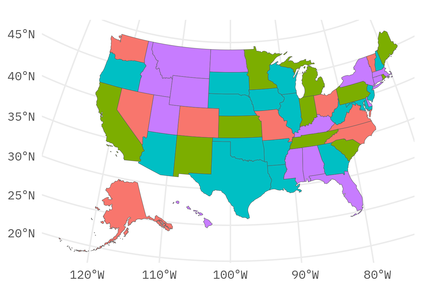
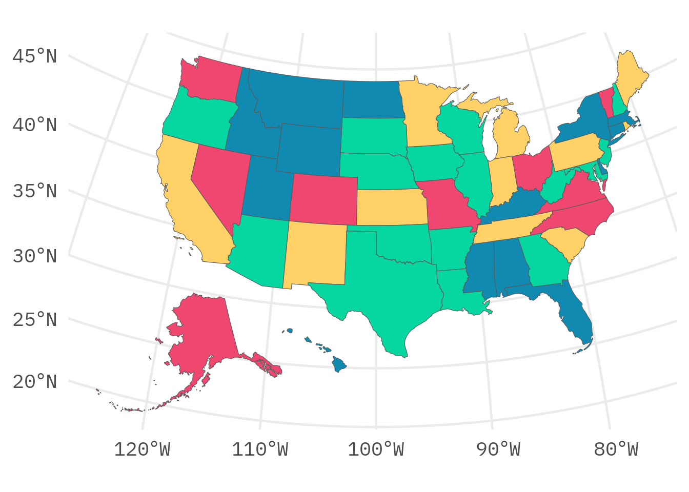
And while we’re at it, we might as well use nicer columns.
grouped_data  |>
  ggplot() +
  geom_sf(aes(fill = group)) +
  theme_minimal(base_size = 18, base_family = 'IBM Plex Mono') +
  theme(legend.position = 'none') +
  scale_fill_manual(
    values = c(
      A = '#ef476f',
      B = '#ffd166',
      C = '#06d6a0',
      D = '#118ab2'
    )
) 
Add patterns
Finally, we can add patterns to our map. This works by using the {ggpattern} package. Basically, all we have to do is replace the geom_sf() layer with geom_sf_pattern().
library(ggpattern)
grouped_data  |>
  ggplot() +
  geom_sf_pattern(aes(fill = group)) +
  theme_minimal(base_size = 18, base_family = 'IBM Plex Mono') +
  theme(legend.position = 'none') +
  scale_fill_manual(
    values = c(
      A = '#ef476f',
      B = '#ffd166',
      C = '#06d6a0',
      D = '#118ab2'
    )
) 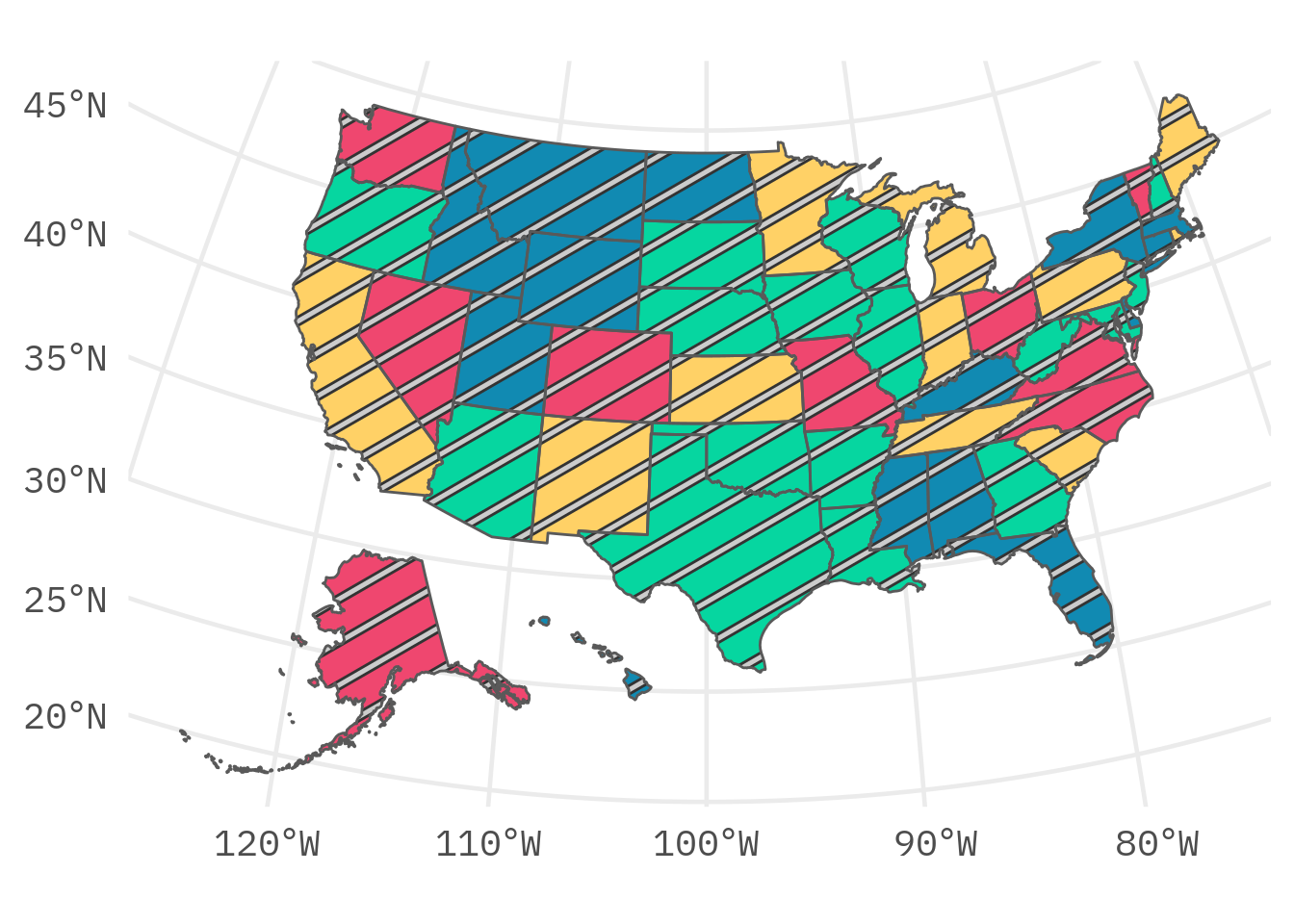
Now, what we get is one pattern for the whole of the US. To change that all we have to do is use the pattern aesthetic from {ggpattern} and map our group column to it.
grouped_data  |>
  ggplot() +
  geom_sf_pattern(
    aes(
      fill = group,
      pattern = group
    )
  ) +
  theme_minimal(base_size = 18, base_family = 'IBM Plex Mono') +
  theme(legend.position = 'none') +
  scale_fill_manual(
    values = c(
      A = '#ef476f',
      B = '#ffd166',
      C = '#06d6a0',
      D = '#118ab2'
    )
) 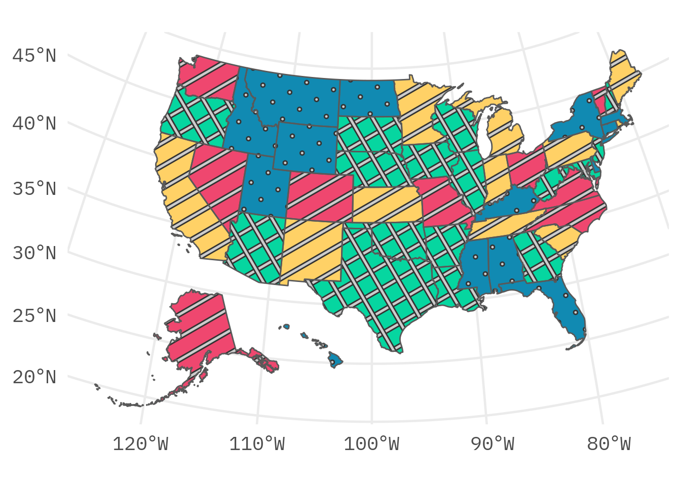
Finally, just as with the fill aesthetic, we can set other values via a scale_*_manual() layer. Here, that’s scale_pattern_manual().
grouped_data  |>
  ggplot() +
  geom_sf_pattern(
    aes(
      fill = group,
      pattern = group
    )
  ) +
  theme_minimal(base_size = 18, base_family = 'IBM Plex Mono') +
  theme(legend.position = 'none') +
  scale_fill_manual(
    values = c(
      A = '#ef476f',
      B = '#ffd166',
      C = '#06d6a0',
      D = '#118ab2'
    )
  ) +
  scale_pattern_manual(
    values = c(
      A = 'stripe',
      B = 'crosshatch',
      C = 'circle',
      D = 'none'
    )
) 
Now that’s a pretty cool map, isn’t it? We could use one of ggpattern’s many extra options like pattern_angle to modify the patterns even further.
grouped_data  |>
  ggplot() +
  geom_sf_pattern(
    aes(
      fill = group,
      pattern = group,
      pattern_angle = group
    )
  ) +
  theme_minimal(base_size = 18, base_family = 'IBM Plex Mono') +
  theme(legend.position = 'none') +
  scale_fill_manual(
    values = c(
      A = '#ef476f',
      B = '#ffd166',
      C = '#06d6a0',
      D = '#118ab2'
    )
  ) +
  scale_pattern_manual(
    values = c(
      A = 'stripe',
      B = 'crosshatch',
      C = 'circle',
      D = 'none'
    )
) 
Conclusion
Nice. We have successfully added patterns to our US map. If you found this helpful, here are some other ways I can help you:
- 3 Minute Wednesdays: A weekly newsletter with bite-sized tips and tricks for R users
- Insightful Data Visualizations for “Uncreative” R Users: A course that teaches you how to leverage
{ggplot2}to make charts that communicate effectively without being a design expert.


