# A tibble: 333 × 4
   sex    body_mass_g species bill_length_mm
   <fct>        <int> <fct>            <dbl>
 1 male          3750 Adelie            39.1
 2 female        3800 Adelie            39.5
 3 female        3250 Adelie            40.3
 4 female        3450 Adelie            36.7
 5 male          3650 Adelie            39.3
 6 female        3625 Adelie            38.9
 7 male          4675 Adelie            39.2
 8 female        3200 Adelie            41.1
 9 male          3800 Adelie            38.6
10 male          4400 Adelie            34.6
# ℹ 323 more rowsThe ultimate beginner’s guide to generalized linear models (GLMs)
Statistics
ML
This is an beginner’s guide on GLMs. We cover the mathematical foundations as well as how to implement GLMs with R. The implementations are done with and without
{tidymodels}.
You may have never heard about generalized linear models (GLMs). But you’ve probably heard about logistic regression or Poisson regression. Both of them are special cases of GLMs.
There are even more special cases of GLMs. That’s because GLMs are versatile statistical models. And in this blog post we’re going to explore the mathematical foundations of these models. Actually, this post is based on one of my recent Twitter threads. You can think of this post as the long form version of that thread.
Here, I’ll add a few more details on the mathematical foundations of GLMs.1 More importantly, though, I will show you how to implement GLMs with R. We’ll learn both the {tidymodels} and the {stats} way of doing GLMs. So without further ado, let’s go.
Logistic regression
Let’s start with logistic regression. Assume that you have the following data about penguins.
Imagine that your goal is to classify penguins as male or female based on the other variables body_mass_g, species and bill_length_mm. Better yet, let’s make this specific. Here’s a dataviz for this exact scenario.
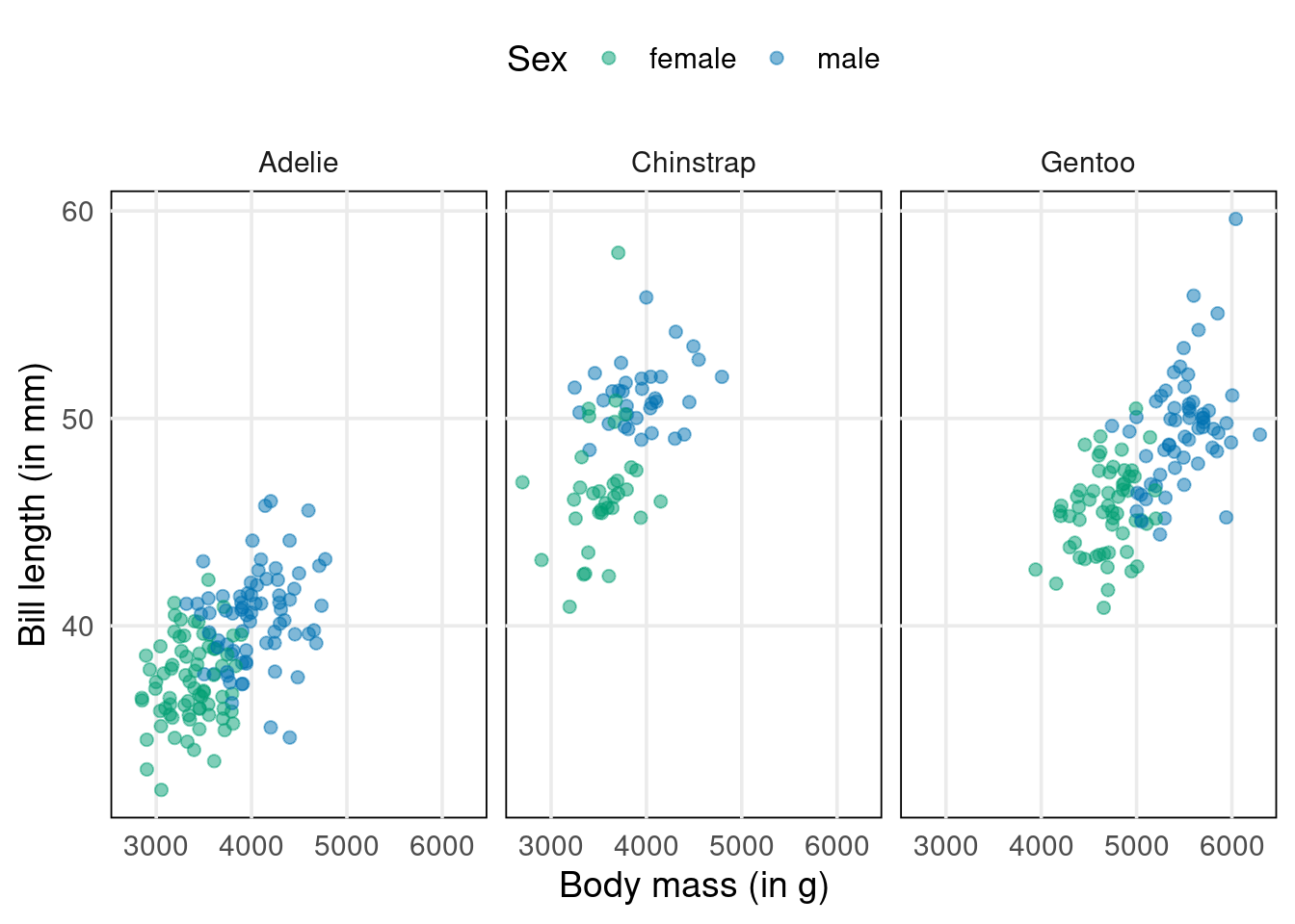
As you can see, the male and female penguins form clusters that do not overlap too much. However, regular linear regression won’t help us to distinguish them. Think about it. Its output is something numerical. Here, we want to find classes.
So, how about trying to predict a related numerical quantity then? Like a probability that a penguin is male. Could we convert the classes to 0 and 1 and then run a linear regression? Well, we could. But this won’t give us probabilities either. Why? Because predictions are not restricted to \([0, 1]\).
But I suspect you’re REALLY determined to use linear regression. After all, what have you learned ordinary least squares (OLS) for if not for using it everywhere? So, what saves you from huge predictions? That’s the glorious logistic function (applied to linear regression’s predictions). It looks like this.
tibble(x = seq(-10, 10, 0.1), y = plogis(x)) %>%
  ggplot(aes(x, y)) +
  geom_line(color = thematic::okabe_ito(3)[3], size = 2) +
  theme_minimal(base_size = 14) +
  theme(panel.grid.minor = element_blank())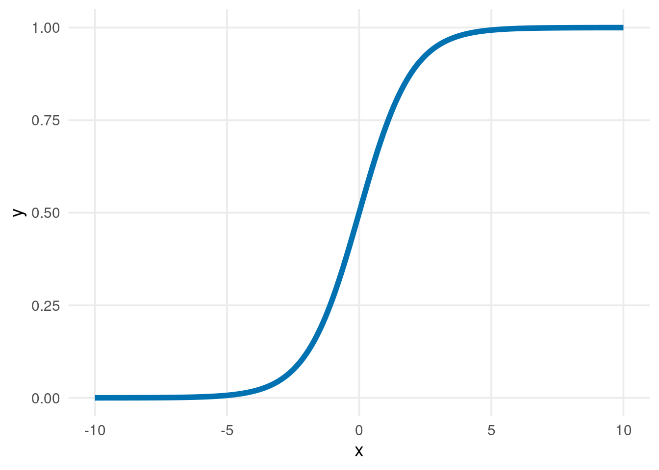
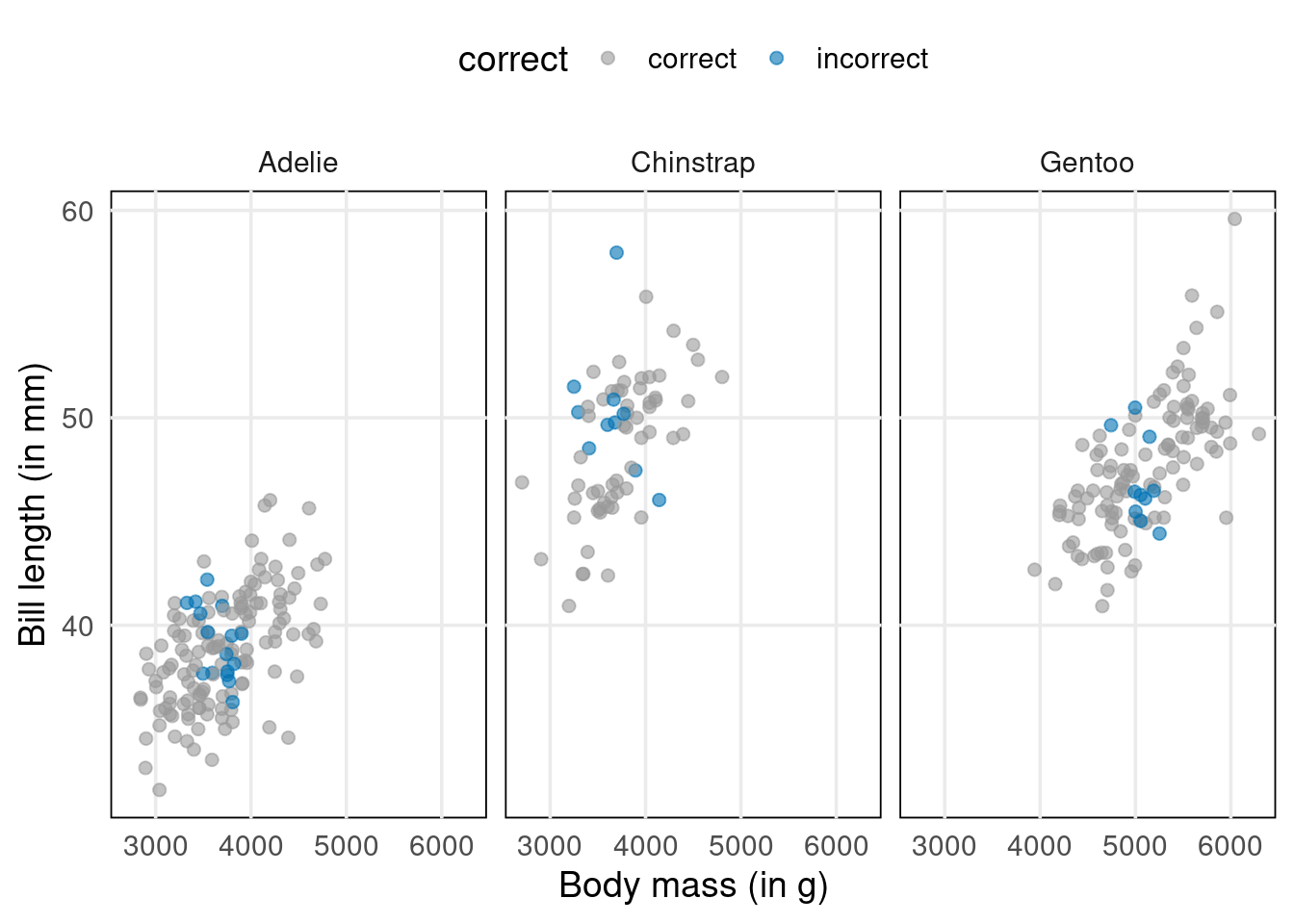
I’ve applied this strategy to our data to “predict” probabilities. Then, I used a 50% threshold for classification.
Note that I have chosen this threshold here only for demo purposes. In general, 50% is not a good threshold. That’s because there are many situations where you want your model to be really sure before it makes a classification. For example, with malignant tumor detection we want to use a threshold that is different from a coin flip. Clearly, we want to be sure that a tumor is dangerous before we undergo surgery.
So, back to our prediction strategy. Against all odds we’ve run a linear regression to “predict” probabilities and classified on this 50% threshold. Does this give us good results? Have a look for yourself.
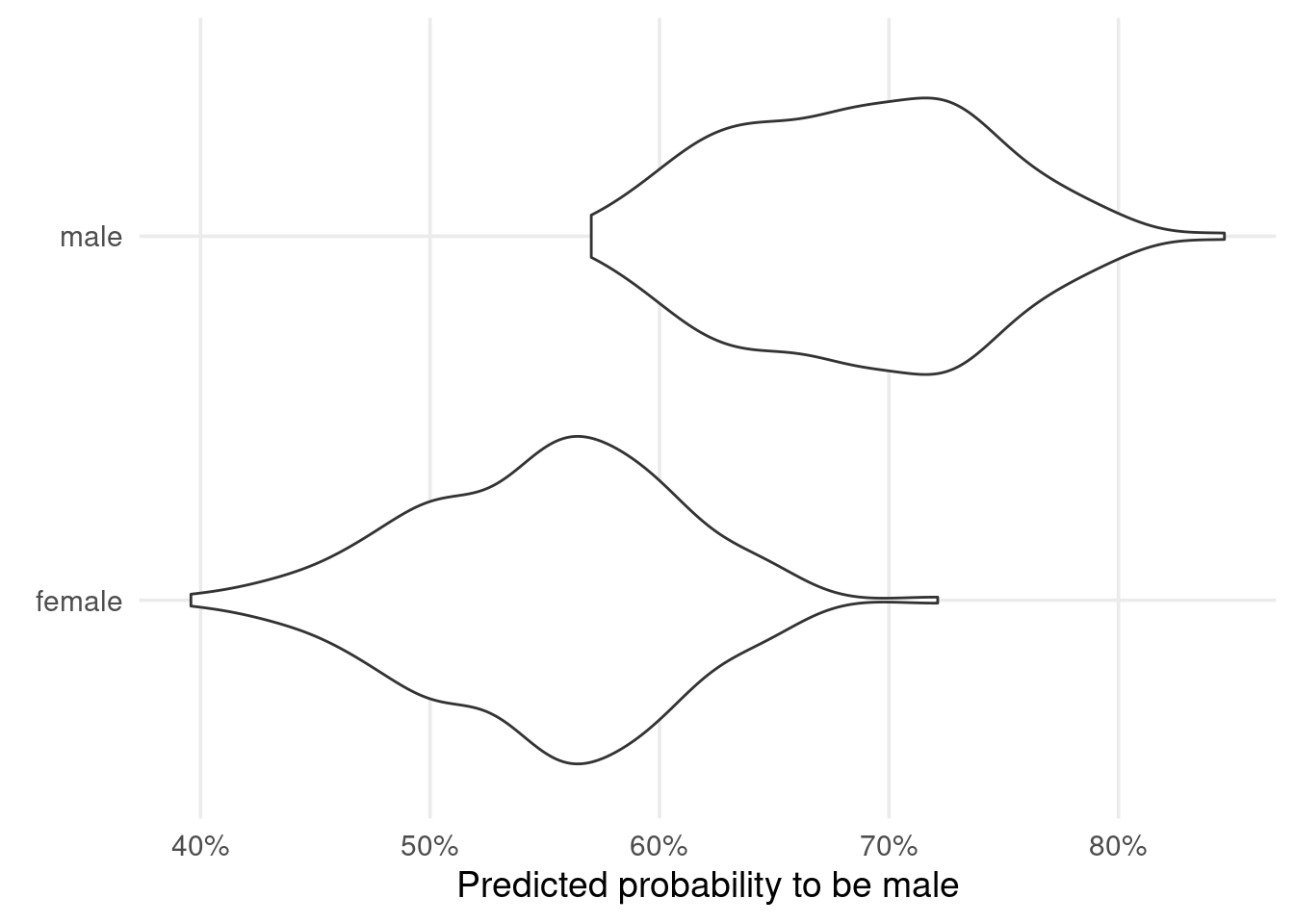

The predictions for male and female penguins overlap quite a lot. This leads to many incorrect classifications. Not bueno. At this point, you may as well have trained a model that answers “Is this a male penguin?” with “Nope, just Chuck Testa”.
So, our classification is bad. And hopefully I’ve convinced you that OLS isn’t the way to go here. But what now?
Well, it wasn’t all bad. The idea of linking a desired quantity (like a probability) to a linear predictor is actually what GLMs do. To make it work, let’s take a step back.
Usually, we model our response variable \(Y\) by decomposing it into
- a deterministic function \(f(X_1,..., X_n)\) dependent on predictors \(X_1, \ldots, X_p\), \(p \in \mathbb{N}\), plus
- a random error term
Thus, regression is nothing but finding a function describing the average outcome. With a little change in notation this becomes clearer:
\[ \begin{align*} Y_i &= f(X_1, \ldots, X_p) + \varepsilon_i \\[2mm] &= \mathbb{E}[Y_i | X_1, \ldots, X_p] + \varepsilon_i, \quad i = 1, \ldots, n \end{align*} \]
In linear regression, this deterministic function is given by a linear predictor. We will denote this linear predictor by \(\eta_i(\beta)\) Note that it depends on a parameter \(\beta \in \mathbb{R}^{p + 1}\).
\[ \eta_i(\beta) = \beta_0 + x_{i, 1}\beta_1 + \cdots + x_{i, p} \beta_p \]
Alright, we’ve emphasized that we’re really trying to model an expectation. Now, think about what we’re trying to predict. We’re looking for probabilities, are we not?
And do we know a distribution whose expectation is a probability? Bingo! We’re thinking about Bernoulli. Therefore, let us assume that our response variable \(Y\) is Bernoulli-distributed (given our predictors), i.e. \(Y_i | X_1, \ldots, X_p \sim \text{Ber}(\pi_i)\).
And now we’re back with our idea to link the average outcome to a linear predictor via a suitable transformation (logistic function). This sets up our model. In formulas, this is written as
\[ \mathbb{E}[Y_i | X_1, \ldots, X_p] = \pi_i = h\big(\eta_i(\beta)\big) \]
where
\[ h(x) = \frac{e^{\text{x}}}{1 + e^x}. \]
You’re thinking we’ve tried this already, aren’t you? How will we get different results? Isn’t this new setup just semantics? Theoretic background is useless in practice, right? (I’ve actually heard someone say that to a speaker at a scientific workshop. A shitshow ensued.)
Previously, we used the OLS estimator to find the linear predictor’s parameter \(\beta\). But with our new model setup comes a new way of estimating \(\beta\). Take a look. Compare the results of using the OLS estimator with what we get when we maximize the so-called likelihood.
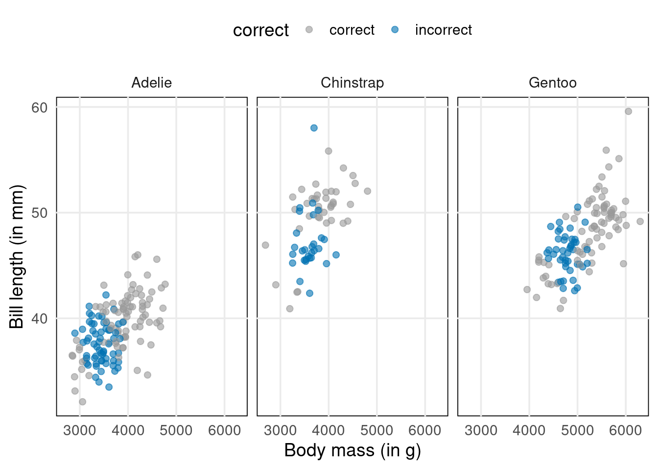
Much fewer incorrect results, right? And that’s despite having used the same 50% threshold once I predicted probabilites. This means that maximizing the likelihood delivers a way better estimator. Let’s see how that works.
The likelihood function \(L\) is the product of the densities of the assumed distribution of Y given the predictors (here Bernoulli). This makes it the joint probability of the observed data. In formulas, this is
\[ L(\beta) := \prod_{i = 1}^n f(y_i | \beta) = \prod_{i = 1}^n \pi_i^{y_i} (1 - \pi_i)^{1 - y_i}. \]
We estimate \(\beta\) by maximizing this function or equivalently (but easier) its logarithm
\[ l(\beta) := \log L(\beta) = \sum_{i = 1}^n \bigg[ \underbrace{y_i \log \bigg( \frac{\pi_i}{1 - \pi_i} \bigg) + \log (1 - \pi_i)}_{=: l_i(\beta)} \bigg]. \]
How do we find this maximum? By using the same strategy as for any other function that we want to maximize: Compute the first derivative and find its root. That’s why it’s easier to maximize the log-likelihood (sums are easier to differentiate than products).
In this context, the first derivative2 is also known as score fct
\[ s(\beta) := \frac{\partial l(\beta)}{\partial \beta} = \sum_{i = 1}^n \frac{\partial l_i(\beta)}{\partial \beta} = \sum_{i = 1}^n s_i(\beta), \]
where
\[ \begin{align*} s_i(\beta) &= x_i(y_i - \pi_i) = x_i\big(y_i - h(x_i^T \beta)\big)\quad \text{and} \\[2mm] h(x) &= \frac{e^{\text{x}}}{1 + e^x} \end{align*} \]
Here, finding a root is hard because no analytical solutions exist. Thus, we’ll have to rely on numerical methods.
Newton’s method
A well-known procedure is Newton’s method. In each iteration it tries to get closer to a function’s root by moving along its gradient. Have a look at this GIF from Wikipedia. It shows how Newton’s method works for a univariate function. But the same ideas work in higher dimensions, i.e. in \(\mathbb{R}^n\) where \(n \in \mathbb{N}\).
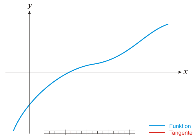
Alright, let me unwrap what you see here. In each iteration, Newton’s method computes \(f(x_k)\), i.e. the function’s value at \(x_k\) (the current value). Then, it uses the function’s derivative \(f^{\prime}\) to find the tangent line of \(f\) at the current position \(x_k\). Once the tangent line is found, our new position \(x_{k + 1}\) is determined by the intersection of the tangent line and the \(x\)-axis. All of this can be summarized via
\[ x_{k + 1} = f(x_k) - (f^{\prime}(x_k))^{-1} f(x_k). \]
As I said, this can be generalized for vector-valued functions \(f\). In that case, \(f^{\prime}\) is a matrix (the so called Hessian matrix) and \((f^{\prime})^{-1}\) is the inverse of that matrix. Like the one-dimensional derivative the Hessian matrix is dependent of the current position \(x_k\).
In the context of GLMs, the current position \(x_k\) is usually denoted with \(\beta_{k}\) and the Hessian
\[ \mathcal{J}(\beta) = - \frac{\partial^2 l(\beta)}{\partial \beta \partial \beta^T} \]
is called observed information Matrix. Once again we can summarize Newton’s algorithm in one single line by
\[ \beta_{t + 1} = \beta_{t} + \mathcal{J}^{-1}(\beta_{t}) s(\beta_{t}). \]
Poisson regression
Congrats! You’ve brushed up on one example of GLMs, namely logistic regression. But GLMs wouldn’t be general if that were all.
Depending on the assumed distribution and the function that links the linear predictor to the expectation, GLMs have many names. Poisson regression is another one.
Poisson regression is a GLM which assumes that Y follows a Poisson distribution (who would have seen that one coming), i.e. \(Y_i | X_1, X_2, X_3 \sim \text{Poi}(\lambda_i)\), \(\lambda_i > 0\). A suitable link function is given by the exponential function
\[ \mathbb{E}[Y_i | X_1, X_2, X_3] = \lambda_i = \exp\big(\eta_i(\beta)\big). \]
This model is used when you try to estimate count data like this.
| Marijuana | Cigarette | Alcohol | Count |
|---|---|---|---|
| yes | yes | yes | 911 |
| no | yes | yes | 538 |
| yes | no | yes | 44 |
| no | no | yes | 456 |
| yes | yes | no | 3 |
| no | yes | no | 43 |
| yes | no | no | 2 |
| no | no | no | 279 |
| Alcohol, Cigarette, and Marijuana Use for High School Seniors; Table 7.3 of Agresti, A (2007). An Introduction to Categorical Data Analysis. | |||
Let’s find the maximum-likelihood estimate \(\hat{\beta}\) for the parameter \(\beta\) of our linear predictor \(\eta_i(\beta)\). Thankfully, the formulas look very similar to logistic regression, i.e.
\[ \begin{align*} l(\beta) &= \sum_{i = 1}^n \big[y_i x_i^T\beta - \exp(x_i^T\beta )\big] \\ s(\beta) &= \sum_{i = 1}^n x_i\big(y_i - \exp(x_i^T \beta)\big) \end{align*} \]
Again, applying Newton’s method to the score function \(s\) will give us its root and therefore the ML-estimate of \(\beta\).
Generalized linear models
We’ve now seen two examples of GLMs. In each case, we have assumed two different distributions and link functions. This begs two questions 🤔
- Does this work with any distribution?
- How in the world do we choose the link function?
The secret ingredient that has been missing is a concept known as exponential families. It can answer both questions. Isn’t that just peachy?
Exponential families (not to be confused with the exponential distribution) are distributions whose density can be rewritten in a very special form
\[ f(y | \theta) = \exp\bigg\{ \frac{y\theta - b(\theta)}{\phi}w + c(y, \phi, w) \bigg\}, \]
where
- \(\theta\) is the natural/canonical parameter
- \(b(\theta)\) is a twice differentiable function
- \(\phi\) is a dispersion parameter
- \(w\) is a known weight
- \(c\) is a normalization constant independent of \(\theta\)
Honestly, this curious form is anything but intuitive. Yet, it is surprisingly versatile and the math just works. If you ask me, that’s quite mathemagical3.
| Distribution | \(\theta\) | \(b(\theta)\) | \(b^\prime(\theta)\) | \(\phi\) |
|---|---|---|---|---|
| \(\mathcal{N}(\mu, \sigma^2)\) | \(\mu\) | \(\theta^2/2\) | \(\theta\) | \(\sigma^2\) |
| \(\text{Ber}(\pi)\) | \(\log (\pi / (1 - \pi))\) | \(\log(1 + e^\theta)\) | \(\frac{e^\theta}{1 + e^\theta}\) | 1 |
| \(\text{Poi}(\lambda)\) | \(\log(\lambda)\) | \(\exp(\theta)\) | \(\exp(\theta)\) | 1 |
It probably doesn’t come as a surprise that Bernoulli and Poisson distributions are exponential families (see table or Wikipedia for even more exponential distributions). But what may surprise you is this:
The function \(b\) plays an extraordinary role: Its derivative can be used as link function! That’s why we have chosen the link function the way we did. In fact, that’s the canoncial choice.
So, now you know GLMs’ ingredients: Exponential families and link functions.
Bam! We’ve made it through the math part. Now begins the programming part.
Implementing GLMs
As promised, we will implement GLMs in two different ways. First, we’ll do it the {stats} way.
GLMs with glm().
With {stats}, the glm() function is the main player to implement any GLM. Among other arguments, this function accepts
- a
formulaargument: This is how we tellglm()what variable we want to predict based on which predictors. - a
familyargument: This is the exponential family that we want to use (for logistic regression this will be Bernoulli or, more generally, binomial) - a
dataargument: This is the data.frame/tibble that contains the variables that you’ve stated in theformula.
For our penguins example, this may look like this.
glm.mod <- glm(
  sex ~ body_mass_g + bill_length_mm + species,
  family = binomial,
  data = penguins_data
)
Here, I’ve saved our fitted model into a variable glm.mod. For our purposes, we can treat this variable like a list that is equipped with a so-called class attribute (which influences the behavior of some functions later). Our list’s column fitted.values contains the probabilities the GLM predicted, e.g.
glm.mod$fitted.values[1:10] 1 2 3 4 5 6 7
0.69330991 0.80620808 0.12555009 0.05499928 0.55937374 0.45142835 0.99939311
8 9 10
0.14437378 0.69994208 0.92478757 Now we can manually turn the predicted probabilities into sex predictions. That requires us to know whether the predicted probability refers to male or female penguins.
Strolling through the docs of glm() reveals that the second level in our response factor sex is considered a “success”. So that means the probability refers to male penguins (because that’s the second level of sex). Tricky, I know.
threshold <- 0.5
preds <- penguins_data %>%
  mutate(
    prob.fit = glm.mod$fitted.values,
    prediction = if_else(prob.fit > threshold, 'male', 'female'),
    correct = if_else(sex == prediction, 'correct', 'incorrect')
  )
preds
# A tibble: 333 × 7
sex body_mass_g species bill_length_mm prob.fit prediction correct
<fct> <int> <fct> <dbl> <dbl> <chr> <chr>
1 male 3750 Adelie 39.1 0.693 male correct
2 female 3800 Adelie 39.5 0.806 male incorrect
3 female 3250 Adelie 40.3 0.126 female correct
4 female 3450 Adelie 36.7 0.0550 female correct
5 male 3650 Adelie 39.3 0.559 male correct
6 female 3625 Adelie 38.9 0.451 female correct
7 male 4675 Adelie 39.2 0.999 male correct
8 female 3200 Adelie 41.1 0.144 female correct
9 male 3800 Adelie 38.6 0.700 male correct
10 male 4400 Adelie 34.6 0.925 male correct
# ℹ 323 more rowsAnd we can also predict other probabilities for observations that have not been present in the original dataset.
new_observations <- tibble(
  body_mass_g = c(4532, 5392),
  bill_length_mm = c(40, 49),
  species = c('Adelie', 'Gentoo')
)
predict(
  glm.mod,
  newdata = new_observations
)
1 2
6.911824 3.661797 Note that this gave us the value of the linear predictors. But that’s not we’re interested, right? So let’s tell predict() that we care about the response variable.
predict(
  glm.mod,
  newdata = new_observations,
  type = 'response'
)
1 2
0.9990051 0.9749570 Now, these look more like probabilities. And they are. These are our predicted probabilities. But we can also save the probabilities into our tibble.
new_observations |>
  mutate(
    pred_prob = predict(
      glm.mod,
      newdata = new_observations,
      type = 'response'
    )
  )
# A tibble: 2 × 4
body_mass_g bill_length_mm species pred_prob
<dbl> <dbl> <chr> <dbl>
1 4532 40 Adelie 0.999
2 5392 49 Gentoo 0.975One last thing before we move on to {tidymodels}. At first, it may be hard to work with predict() because the documentation does not feel super helpful at first. Take a look. The docs do not tell you much about arguments like newdata or type.

That’s because predict() is actually a really versatile function. It works differently depending on what kind of model object you feed it with, e.g. output from lm() or glm(). That’s the part that is determined by glm.mod’s class attribute.
Now, at the end of predict()’s docs you will find a list that shows you all kinds of other predict() functions like predict.glm(). This is the function that works with objects of class glm. In the docs of the latter function you can now look up all arguments that you need.
GLMs with {tidymodels}
Like the tidyverse, {tidymodels} is actually more than a single package. It is a whole ecosystem of packages. All of these packages share a design philosophy and are tailored to modelling/machine learning. Check out how many packages get attached when we call {tidymodels}.
library(tidymodels)── Attaching packages ────────────────────────────────────── tidymodels 1.1.0 ──✔ broom 1.0.4 ✔ rsample 1.1.1
✔ dials 1.2.0 ✔ tune 1.1.1
✔ infer 1.0.4 ✔ workflows 1.1.3
✔ modeldata 1.1.0 ✔ workflowsets 1.0.1
✔ parsnip 1.1.0 ✔ yardstick 1.2.0
✔ recipes 1.0.6 ── Conflicts ───────────────────────────────────────── tidymodels_conflicts() ──
✖ scales::discard() masks purrr::discard()
✖ dplyr::filter() masks stats::filter()
✖ recipes::fixed() masks stringr::fixed()
✖ dplyr::lag() masks stats::lag()
✖ yardstick::spec() masks readr::spec()
✖ recipes::step() masks stats::step()
• Search for functions across packages at https://www.tidymodels.org/find/Obviously, we can’t dig into everything here. So, let’s just cover the minimal amount we need for our use case. For a more detailed intro to {tidymodels} you can check out my YARDS lecture notes. And for a really thorough deep dive I recommend the Tidy Modeling with R book.
To run a logistic regression in the {tidymodels} framework we need to first define a model specification. These are handled by {parsnip}. Here, this looks like this.
logistic_spec <- logistic_reg() %>%
  set_engine("glm") %>%
  set_mode("classification")
logistic_spec
Logistic Regression Model Specification (classification)
Computational engine: glm Notice that the output is really nothing more than a description saying
- we’re doing a logistic regression (
logistic_reg()). - we want to use the
stats::glm()engine/function to fit the logistic regression (set_engine("glm")) - we want to do classification (and not regression) (
set_mode("classification"))
Notice that there are other engines that we could use, e.g. "glmnet" or "keras". Also, specifying the mode is kind of superfluous here. But for models that can do both, classification and regression, e.g. random forests, this is necessary. That’s why I’ve shown that step here.
Alright, so we’ve set up our model. Time to fit it. That happens with fit().
glm.tidymod <- logistic_spec |>
  fit(
    formula = sex ~ body_mass_g + bill_length_mm + species,
    data = penguins_data
  )
Like predict(), the fit() function works a little bit differently depending on its input object. What’s more is that can be a bit tricky to find the correct page in the docs to look up the correct arguments. What you’re actually looking for is fit.model_spec(). That’s because logistic_spec is not a glm object but a model_spec object.
Don’t worry about the technicalities if you’ve found that confusing. The point is that fit() expects a
- model specification
- a formula (exactly like
glm()) - data
Now we can throw glm.tidymod into predict(). Beware of your objects though! In the {stats} way, we’ve passed a glm object to predict so really it behaves like predict.glm(). Now, we’re using a model_fit() object (that’s what fit() returns). So, we’ll need to look at the docs of predict.model_fit().
Et voilà! The documentation reveals that there are arguments called new_data (mind the _) and type. The latter argument can deal with a lot of different inputs. But here we’re just going with "prob".
new_observations |>
  mutate(
    pred_prob = predict(
      glm.tidymod,
      new_data = new_observations,
      type = 'prob'
    )
  )
# A tibble: 2 × 4
body_mass_g bill_length_mm species pred_prob$.pred_female $.pred_male
<dbl> <dbl> <chr> <dbl> <dbl>
1 4532 40 Adelie 0.000995 0.999
2 5392 49 Gentoo 0.0250 0.975Notice that this actually returns two probabilities. One for each sex. That’s great because we don’t have to wonder anymore what class our predicted probability refers to.
This is just one of many advantages working with {tidymodels}. You will still need some knowledge of the engine you’re using (glm() in this case). But {tidymodels} will give you a nicer interface to the engine. And you can easily switch between engines and other models because it’s all constructed from a unified interface.
Finally, let me mention that switching to a Poisson regression is just a matter of exchanging logistic_reg() for poisson_reg() (and changing the mode to "regression"). In fact, that’s how you switch to any other model, e.g. to random forests via rand_forest().
Conclusion
That’s a wrap! This guide should give you a solid understanding of both, the theoretical and practical, aspects of GLMs. If you’ve got any questions, feel free to use the comment section or send me a mail.
If you don’t want to stay in touch or don’t want to miss new blog posts, then don’t forget to subscribe to my newsletter below. Enjoy the rest of your day and see you next time!
References
Fahrmeir, Ludwig, Thomas Kneib, Stefan Lang, and Brian Marx. 2013. Regression. Springer Berlin Heidelberg. https://doi.org/10.1007/978-3-642-34333-9.
Footnotes
Of course I can’t cover everything. This is a beginner’s guide after all. For more details let me refer to the excellent book (Fahrmeir et al. 2013).↩︎
For detailed calculations of the score function and any other formula, I recommend that you refer to (Fahrmeir et al. 2013).↩︎
An interesting perspective on what makes exponential familes so magical can be found on SE.↩︎


