library(tidyverse)
df <- read_csv('tbl_data.csv')
df
## # A tibble: 14 × 7
##    stock_symbol company          change_abs change_rel percent open2020 open2022
##    <chr>        <chr>                 <dbl>      <dbl> <chr>      <dbl>    <dbl>
##  1 INTC         Intel Corporati…    -34.5     -0.572   -57.22%     60.2     25.8
##  2 META         Meta Platforms,…    -90.3     -0.437   -43.70%    207.     116.
##  3 CRM          Salesforce, Inc.    -34.2     -0.209   -20.88%    164.     130.
##  4 NFLX         Netflix, Inc.       -42.9     -0.132   -13.16%    326.     283.
##  5 AMZN         Amazon.com, Inc.    -10.9     -0.116   -11.61%     93.8     82.9
##  6 CSCO         Cisco Systems, …     -0.800   -0.0166  -1.66%      48.1     47.3
##  7 ADBE         Adobe Inc.            0.75     0.00227 0.23%      330      331.
##  8 IBM          International B…     11.5      0.0892  8.92%      129.     141.
##  9 GOOGL        Alphabet Inc.        19.2      0.285   28.48%      67.4     86.6
## 10 MSFT         Microsoft Corpo…     76.9      0.484   48.41%     159.     236.
## 11 ORCL         Oracle Corporat…     27.7      0.520   52.00%      53.3     81.0
## 12 AAPL         Apple Inc.           53.9      0.728   72.82%      74.1    128.
## 13 NVDA         NVIDIA Corporat…     84.3      1.41    141.29%     59.7    144.
## 14 TSLA Tesla, Inc. 92.1 3.25 325.41% 28.3 120.Create engaging tables with R or Python using {gt}
This blog post is two posts in one. I’m showing you how to create engaging tables with R and Python through a unified interface.
The {gt} package is a beloved package in R that allows users to create engaging tables. This package does so through a structured and easy to learn syntax. And the cool thing is that {gt} and its excellent syntax for creating tables is now available for Python too under the name great_tables. So in this blog post, I’m showing you how to create an engaging table with more or less the same syntax in R and Python.
And as always, this blog post is available as a video on YouTube too. Here’s the R version:
And for the Python version, check out this video:
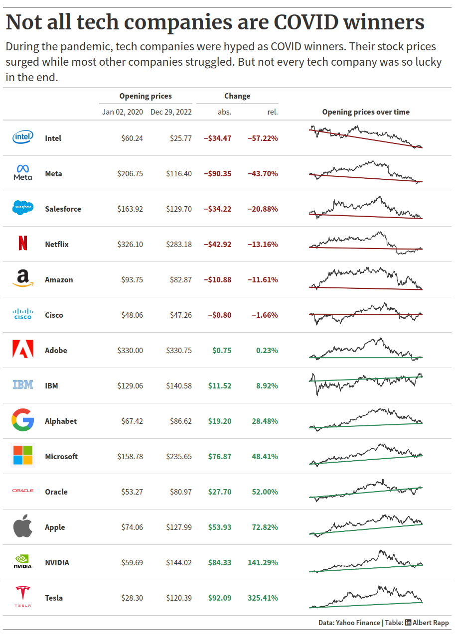
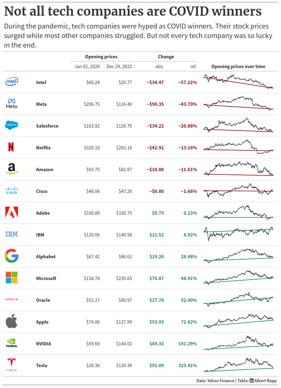
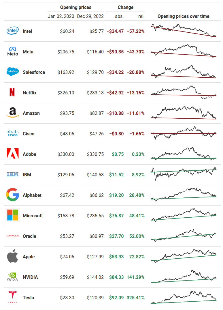
What we’re going for
In this blog post, we’re going to create the following two tables:
The data set
The data set that we’re going to use comes from TidyTuesday. In this post, we’re not going to worry about how to calculate all of the numbers that we see in the above tables. Instead, we’re just going to assume that we have a csv with all the data pre-processed already. You can get that file here.
import polars as pl
# Set amount of rows that will be displayed to 30
pl.Config.set_tbl_rows(30)
## <class 'polars.config.Config'>

df = pl.read_csv('tbl_data.csv')
df
shape: (14, 7)
| stock_symbol | company | change_abs | change_rel | percent | open2020 | open2022 |
|---|---|---|---|---|---|---|
| str | str | f64 | f64 | str | f64 | f64 |
| "INTC" | "Intel Corporat… | -34.470002 | -0.572211 | "-57.22%" | 60.240002 | 25.77 |
| "META" | "Meta Platforms… | -90.349998 | -0.437001 | "-43.70%" | 206.75 | 116.400002 |
| "CRM" | "Salesforce, In… | -34.220001 | -0.20876 | "-20.88%" | 163.919998 | 129.699997 |
| "NFLX" | "Netflix, Inc." | -42.920013 | -0.131616 | "-13.16%" | 326.100006 | 283.179993 |
| "AMZN" | "Amazon.com, In… | -10.879997 | -0.116053 | "-11.61%" | 93.75 | 82.870003 |
| "CSCO" | "Cisco Systems,… | -0.800003 | -0.016646 | "-1.66%" | 48.060001 | 47.259998 |
| "ADBE" | "Adobe Inc." | 0.75 | 0.002273 | "0.23%" | 330.0 | 330.75 |
| "IBM" | "International … | 11.516907 | 0.089235 | "8.92%" | 129.063095 | 140.580002 |
| "GOOGL" | "Alphabet Inc." | 19.199501 | 0.284772 | "28.48%" | 67.420502 | 86.620003 |
| "MSFT" | "Microsoft Corp… | 76.869995 | 0.484129 | "48.41%" | 158.779999 | 235.649994 |
| "ORCL" | "Oracle Corpora… | 27.700001 | 0.519993 | "52.00%" | 53.27 | 80.970001 |
| "AAPL" | "Apple Inc." | 53.93 | 0.728193 | "72.82%" | 74.059998 | 127.989998 |
| "NVDA" | "NVIDIA Corpora… | 84.332504 | 1.412901 | "141.29%" | 59.6875 | 144.020004 |
| "TSLA" | "Tesla, Inc." | 92.09 | 3.254064 | "325.41%" | 28.299999 | 120.389999 |
Get image paths
Notice that these data sets do not contain any information about the company logos or the charts in the “Opening prices over time” column. Let’s add that information to the data set. For the company logos, let us thank Tanya Shapiro for curating all of the company images in a GitHub repository that we can use. In particular, note that all files in that repository are named after the stock symbol abbreviatons. So we can get the right image paths by just iterating over the stock_symbol column.
base_url <-  "https://raw.githubusercontent.com/tashapiro/TidyTuesday/master/2023/W6/logos/"

df |>
  mutate(
    logo = glue::glue(
      '<img height=50 src="{base_url}{stock_symbol}.png"></img>'
    )
  ) |>
  # Select columns for better readability
  select(stock_symbol, logo)
## # A tibble: 14 × 2
##    stock_symbol logo
##    <chr>        <glue>
##  1 INTC         <img height=50 src="https://raw.githubusercontent.com/tashapiro…
##  2 META         <img height=50 src="https://raw.githubusercontent.com/tashapiro…
##  3 CRM          <img height=50 src="https://raw.githubusercontent.com/tashapiro…
##  4 NFLX         <img height=50 src="https://raw.githubusercontent.com/tashapiro…
##  5 AMZN         <img height=50 src="https://raw.githubusercontent.com/tashapiro…
##  6 CSCO         <img height=50 src="https://raw.githubusercontent.com/tashapiro…
##  7 ADBE         <img height=50 src="https://raw.githubusercontent.com/tashapiro…
##  8 IBM          <img height=50 src="https://raw.githubusercontent.com/tashapiro…
##  9 GOOGL        <img height=50 src="https://raw.githubusercontent.com/tashapiro…
## 10 MSFT         <img height=50 src="https://raw.githubusercontent.com/tashapiro…
## 11 ORCL         <img height=50 src="https://raw.githubusercontent.com/tashapiro…
## 12 AAPL         <img height=50 src="https://raw.githubusercontent.com/tashapiro…
## 13 NVDA         <img height=50 src="https://raw.githubusercontent.com/tashapiro…
## 14 TSLA         <img height=50 src="https://raw.githubusercontent.com/tashapiro…
base_url = "https://raw.githubusercontent.com/tashapiro/TidyTuesday/master/2023/W6/logos/"
(
df
.with_columns(
(
pl.lit(f'<img height=50 src="{base_url}')
+ pl.col("stock_symbol")
+ pl.lit('.png"></img>')
).alias("logo")
)
# Select columns for better readability
.select("stock_symbol", "logo")
)
shape: (14, 2)
| stock_symbol | logo |
|---|---|
| str | str |
| "INTC" | "<img height=50… |
| "META" | "<img height=50… |
| "CRM" | "<img height=50… |
| "NFLX" | "<img height=50… |
| "AMZN" | "<img height=50… |
| "CSCO" | "<img height=50… |
| "ADBE" | "<img height=50… |
| "IBM" | "<img height=50… |
| "GOOGL" | "<img height=50… |
| "MSFT" | "<img height=50… |
| "ORCL" | "<img height=50… |
| "AAPL" | "<img height=50… |
| "NVDA" | "<img height=50… |
| "TSLA" | "<img height=50… |
Notice how in both cases we have wrapped the url including the stock symbol into <img src=...> tags. That’s a bit of html magic to make sure that our images are displayed later on. Similarly, we can include the paths to the line charts. For this blog post, we assume that these have been saved into png-files in a directory called lines.
df |>
  mutate(
    logo = glue::glue(
      '<img height=50 src="{base_url}{stock_symbol}.png"></img>'
    ),
    stock_symbol = glue::glue(
      '<img height=50 src="lines/{stock_symbol}.png"></img>'
    )
  ) |>
  # Select columns for better readability
  select(stock_symbol, logo)
## # A tibble: 14 × 2
##    stock_symbol                                logo
##    <glue>                                      <glue>
##  1 <img height=50 src="lines/INTC.png"></img>  <img height=50 src="https://raw.…
##  2 <img height=50 src="lines/META.png"></img>  <img height=50 src="https://raw.…
##  3 <img height=50 src="lines/CRM.png"></img>   <img height=50 src="https://raw.…
##  4 <img height=50 src="lines/NFLX.png"></img>  <img height=50 src="https://raw.…
##  5 <img height=50 src="lines/AMZN.png"></img>  <img height=50 src="https://raw.…
##  6 <img height=50 src="lines/CSCO.png"></img>  <img height=50 src="https://raw.…
##  7 <img height=50 src="lines/ADBE.png"></img>  <img height=50 src="https://raw.…
##  8 <img height=50 src="lines/IBM.png"></img>   <img height=50 src="https://raw.…
##  9 <img height=50 src="lines/GOOGL.png"></img> <img height=50 src="https://raw.…
## 10 <img height=50 src="lines/MSFT.png"></img>  <img height=50 src="https://raw.…
## 11 <img height=50 src="lines/ORCL.png"></img>  <img height=50 src="https://raw.…
## 12 <img height=50 src="lines/AAPL.png"></img>  <img height=50 src="https://raw.…
## 13 <img height=50 src="lines/NVDA.png"></img>  <img height=50 src="https://raw.…
## 14 <img height=50 src="lines/TSLA.png"></img>  <img height=50 src="https://raw.…
(
df
.with_columns(
(
pl.lit(f'<img height=50 src="{base_url}')
+ pl.col("stock_symbol")
+ pl.lit('.png"></img>')
).alias("logo"),
(
pl.lit(f'<img height=50 src="lines/')
+ pl.col("stock_symbol")
+ pl.lit('.png"></img>')
).alias("stock_symbol")
)
# Select columns for better readability
.select("stock_symbol", "logo")
)
shape: (14, 2)
| stock_symbol | logo |
|---|---|
| str | str |
| "<img height=50… | "<img height=50… |
| "<img height=50… | "<img height=50… |
| "<img height=50… | "<img height=50… |
| "<img height=50… | "<img height=50… |
| "<img height=50… | "<img height=50… |
| "<img height=50… | "<img height=50… |
| "<img height=50… | "<img height=50… |
| "<img height=50… | "<img height=50… |
| "<img height=50… | "<img height=50… |
| "<img height=50… | "<img height=50… |
| "<img height=50… | "<img height=50… |
| "<img height=50… | "<img height=50… |
| "<img height=50… | "<img height=50… |
| "<img height=50… | "<img height=50… |
Clean up company names
Notice that in the final images the company names are short and concise. Something like International Business Machines is IBM and Apple Inc. is just Apple. This doesn’t happen my accident. We can make that happen with a bit of text cleaning using regular expressions.
df |>
  mutate(
    logo = glue::glue(
      '<img height=50 src="{base_url}{stock_symbol}.png"></img>'
    ),
    stock_symbol = glue::glue(
      '<img height=50 src="lines/{stock_symbol}.png"></img>'
    ),
    company = if_else(
      str_detect(stock_symbol, 'IBM'),
      'IBM',
      company
    ),
    company = str_remove(company, '(,)? Inc\\.'),
    company = str_remove(company, ' (Corporation|Platforms|Systems)'),
    company = str_remove(company, '\\.com')
  ) |>
  # Select columns for better readability
  select(company)
## # A tibble: 14 × 1
##    company
##    <chr>
##  1 Intel
##  2 Meta
##  3 Salesforce
##  4 Netflix
##  5 Amazon
##  6 Cisco
##  7 Adobe
##  8 IBM
##  9 Alphabet
## 10 Microsoft
## 11 Oracle
## 12 Apple
## 13 NVIDIA
## 14 Tesla
(
df
.with_columns(
(
pl.lit(f'<img height=50 src="{base_url}')
+ pl.col("stock_symbol")
+ pl.lit('.png"></img>')
).alias("logo"),
(
pl.lit(f'<img height=50 src="lines/')
+ pl.col("stock_symbol")
+ pl.lit('.png"></img>')
).alias("stock_symbol"),
pl.when(pl.col("stock_symbol").str.contains("IBM"))
.then("IBM")
.otherwise(pl.col("company"))
.str.replace_all(r"(,)? Inc\.", "")
.str.replace_all(r" (Corporation|Platforms|Systems)", "")
.str.replace_all(r"\.com", "")
.alias("company")
)
# Select columns for better readability
.select("company")
)
shape: (14, 1)
| company |
|---|
| str |
| "Intel" |
| "Meta" |
| "Salesforce" |
| "Netflix" |
| "Amazon" |
| "Cisco" |
| "Adobe" |
| "IBM" |
| "Alphabet" |
| "Microsoft" |
| "Oracle" |
| "Apple" |
| "NVIDIA" |
| "Tesla" |
Select columns in desired order
Excellent. Now, we only have to select the columns we need for the table in the order that they appear in the final image.
df_cleaned <- df |>
  mutate(
    logo = glue::glue(
      '<img height=50 src="{base_url}{stock_symbol}.png"></img>'
    ),
    stock_symbol = glue::glue(
      '<img height=50 src="lines/{stock_symbol}.png"></img>'
    ),
    company = if_else(
      str_detect(stock_symbol, 'IBM'),
      'IBM',
      company
    ),
    company = str_remove(company, '(,)? Inc\\.'),
    company = str_remove(company, ' (Corporation|Platforms|Systems)'),
    company = str_remove(company, '\\.com')
  ) |>
  select(
    logo, company, open2020, open2022,
    change_abs, change_rel, stock_symbol
  )
df_cleaned
## # A tibble: 14 × 7
##    logo             company open2020 open2022 change_abs change_rel stock_symbol
##    <glue>           <chr>      <dbl>    <dbl>      <dbl>      <dbl> <glue>
##  1 <img height=50 … Intel       60.2     25.8    -34.5     -0.572   <img height…
##  2 <img height=50 … Meta       207.     116.     -90.3     -0.437   <img height…
##  3 <img height=50 … Salesf…    164.     130.     -34.2     -0.209   <img height…
##  4 <img height=50 … Netflix    326.     283.     -42.9     -0.132   <img height…
##  5 <img height=50 … Amazon      93.8     82.9    -10.9     -0.116   <img height…
##  6 <img height=50 … Cisco       48.1     47.3     -0.800   -0.0166  <img height…
##  7 <img height=50 … Adobe      330      331.       0.75     0.00227 <img height…
##  8 <img height=50 … IBM        129.     141.      11.5      0.0892  <img height…
##  9 <img height=50 … Alphab…     67.4     86.6     19.2      0.285   <img height…
## 10 <img height=50 … Micros…    159.     236.      76.9      0.484   <img height…
## 11 <img height=50 … Oracle      53.3     81.0     27.7      0.520   <img height…
## 12 <img height=50 … Apple       74.1    128.      53.9      0.728   <img height…
## 13 <img height=50 … NVIDIA      59.7    144.      84.3      1.41    <img height…
## 14 <img height=50 … Tesla       28.3    120.      92.1      3.25    <img height…
base_url = "https://raw.githubusercontent.com/tashapiro/TidyTuesday/master/2023/W6/logos/"
df_cleaned = (
df
.with_columns(
(
pl.lit(f'<img height=50 src="{base_url}')
+ pl.col("stock_symbol")
+ pl.lit('.png"></img>')
).alias("logo"),
(
pl.lit(f'<img height=50 src="lines/')
+ pl.col("stock_symbol")
+ pl.lit('.png"></img>')
).alias("stock_symbol"),
pl.when(pl.col("stock_symbol").str.contains("IBM"))
.then("IBM")
.otherwise(pl.col("company"))
.str.replace_all(r"(,)? Inc\.", "")
.str.replace_all(r" (Corporation|Platforms|Systems)", "")
.str.replace_all(r"\.com", "")
.alias("company")
)
.select(
"logo", "company", "open2020", "open2022",
"change_abs", "change_rel", "stock_symbol"
)
)
df_cleaned
shape: (14, 7)
| logo | company | open2020 | open2022 | change_abs | change_rel | stock_symbol |
|---|---|---|---|---|---|---|
| str | str | f64 | f64 | f64 | f64 | str |
| "<img height=50… | "Intel" | 60.240002 | 25.77 | -34.470002 | -0.572211 | "<img height=50… |
| "<img height=50… | "Meta" | 206.75 | 116.400002 | -90.349998 | -0.437001 | "<img height=50… |
| "<img height=50… | "Salesforce" | 163.919998 | 129.699997 | -34.220001 | -0.20876 | "<img height=50… |
| "<img height=50… | "Netflix" | 326.100006 | 283.179993 | -42.920013 | -0.131616 | "<img height=50… |
| "<img height=50… | "Amazon" | 93.75 | 82.870003 | -10.879997 | -0.116053 | "<img height=50… |
| "<img height=50… | "Cisco" | 48.060001 | 47.259998 | -0.800003 | -0.016646 | "<img height=50… |
| "<img height=50… | "Adobe" | 330.0 | 330.75 | 0.75 | 0.002273 | "<img height=50… |
| "<img height=50… | "IBM" | 129.063095 | 140.580002 | 11.516907 | 0.089235 | "<img height=50… |
| "<img height=50… | "Alphabet" | 67.420502 | 86.620003 | 19.199501 | 0.284772 | "<img height=50… |
| "<img height=50… | "Microsoft" | 158.779999 | 235.649994 | 76.869995 | 0.484129 | "<img height=50… |
| "<img height=50… | "Oracle" | 53.27 | 80.970001 | 27.700001 | 0.519993 | "<img height=50… |
| "<img height=50… | "Apple" | 74.059998 | 127.989998 | 53.93 | 0.728193 | "<img height=50… |
| "<img height=50… | "NVIDIA" | 59.6875 | 144.020004 | 84.332504 | 1.412901 | "<img height=50… |
| "<img height=50… | "Tesla" | 28.299999 | 120.389999 | 92.09 | 3.254064 | "<img height=50… |
Create first table with {gt}
Nice. We have the hard data cleaning part done. Now we can focus on creating the tables. The first step is very easy. We just have to pass our cleaned data set to the gt() resp. GT() function.
library(gt)
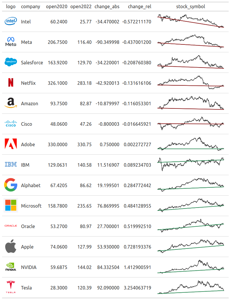
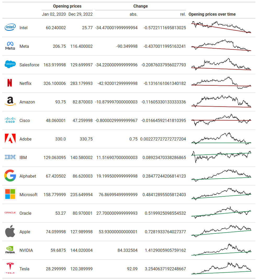
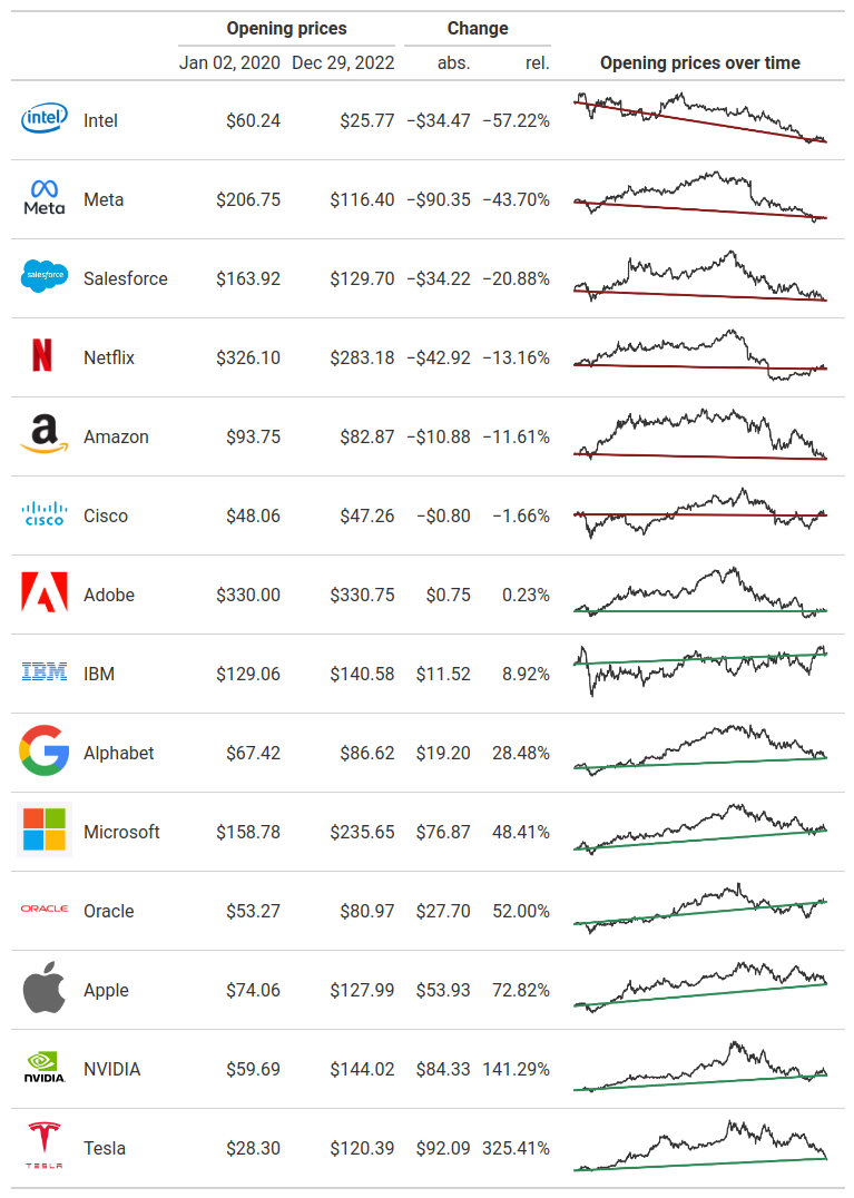
gt(df_cleaned)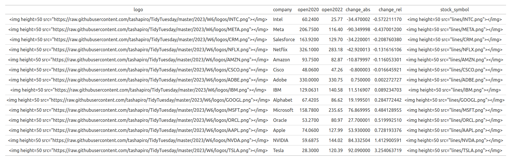
import great_tables as gt
gt.GT(df_cleaned)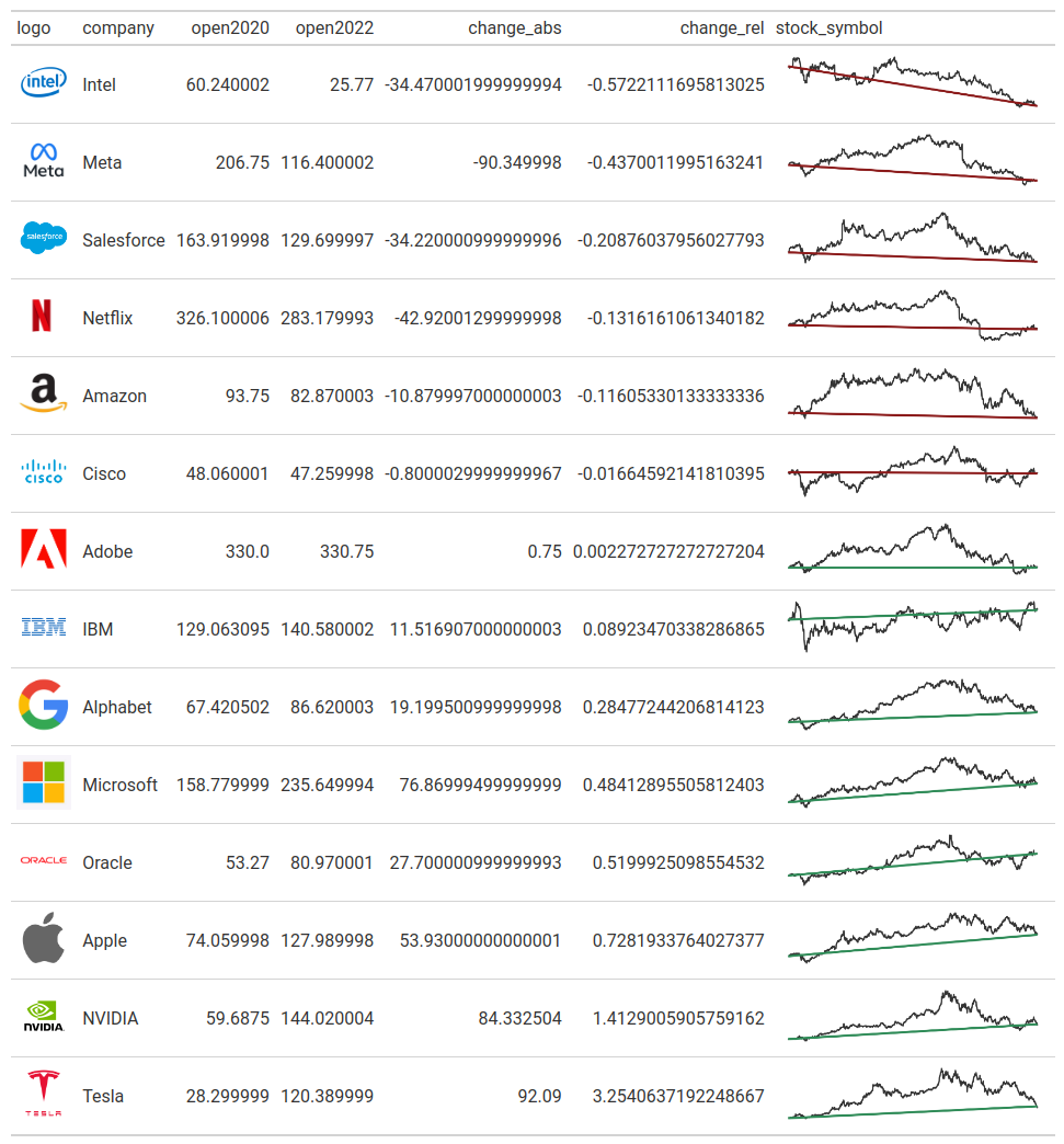
Render images
As you can see, the Python version automatically turns the <img> tags into images. The R version just displays them as text. To fix that in the R version, we can pass the table to fmt_markdown() to format columns as Markdown (which accepts HTML as well.)
library(gt)
df_cleaned |>
  gt() |>
  fmt_markdown(
    columns = c(logo, stock_symbol)
  )
Combine columns with spanners
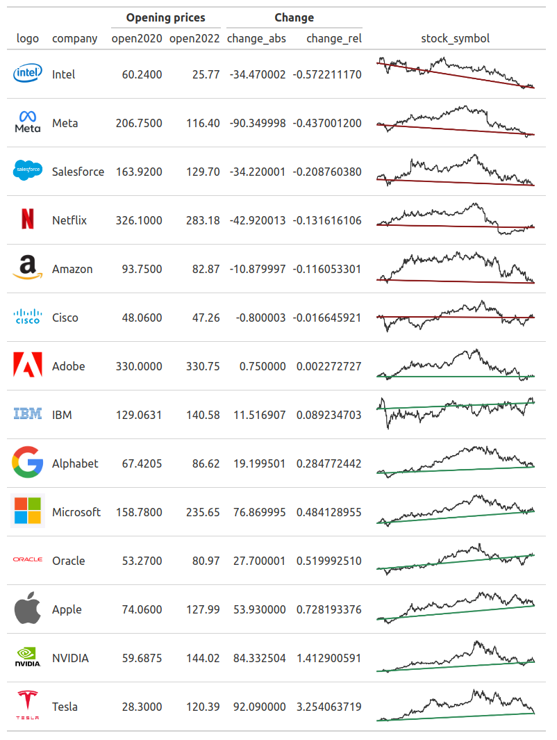
Next, we can combine both the two open prices and the two change columns with tab_spanner(). Here, we can also use the md() function to enable Markdown notation (like using ** for bold text.)
library(gt)
gt(df_cleaned) |>
  fmt_markdown(
    columns = c(logo, stock_symbol)
  ) |>
  tab_spanner(
    label = md('**Opening prices**'),
    columns = c(open2020, open2022)
  ) |>
  tab_spanner(
    label = md('**Change**'),
    columns = c(change_abs, change_rel)
  )
import great_tables as gt
(
  gt.GT(df_cleaned)
  .tab_spanner(
    label = gt.md('**Opening prices**'),
    columns = ["open2020", "open2022"]
  )
  .tab_spanner(
    label = gt.md('**Change**'),
    columns = ["change_abs", "change_rel"]
  )
)
Nicer column labels
Next up are the column labels. We can set them with cols_label().
library(gt)
gt(df_cleaned) |>
  fmt_markdown(
    columns = c(logo, stock_symbol)
  ) |>
  tab_spanner(
    label = md('**Opening prices**'),
    columns = c(open2020, open2022)
  ) |>
  tab_spanner(
    label = md('**Change**'),
    columns = c(change_abs, change_rel)
  ) |>
  cols_label(
    stock_symbol = md('**Opening prices over time**'),
    company = '',
    logo = '',
    open2020 = 'Jan 02, 2020',
    open2022 = 'Dec 29, 2022',
    change_abs = 'abs.',
    change_rel = 'rel.'
  )
import great_tables as gt
(
  gt.GT(df_cleaned)
  .tab_spanner(
    label = gt.md('**Opening prices**'),
    columns = ["open2020", "open2022"]
  )
  .tab_spanner(
    label = gt.md('**Change**'),
    columns = ["change_abs", "change_rel"]
  )
  .cols_label(
        stock_symbol = gt.md('**Opening prices over time**'),
        company = '',
        logo = '',
        open2020 = 'Jan 02, 2020',
        open2022 = 'Dec 29, 2022',
        change_abs = 'abs.',
        change_rel = 'rel.'
    )
)
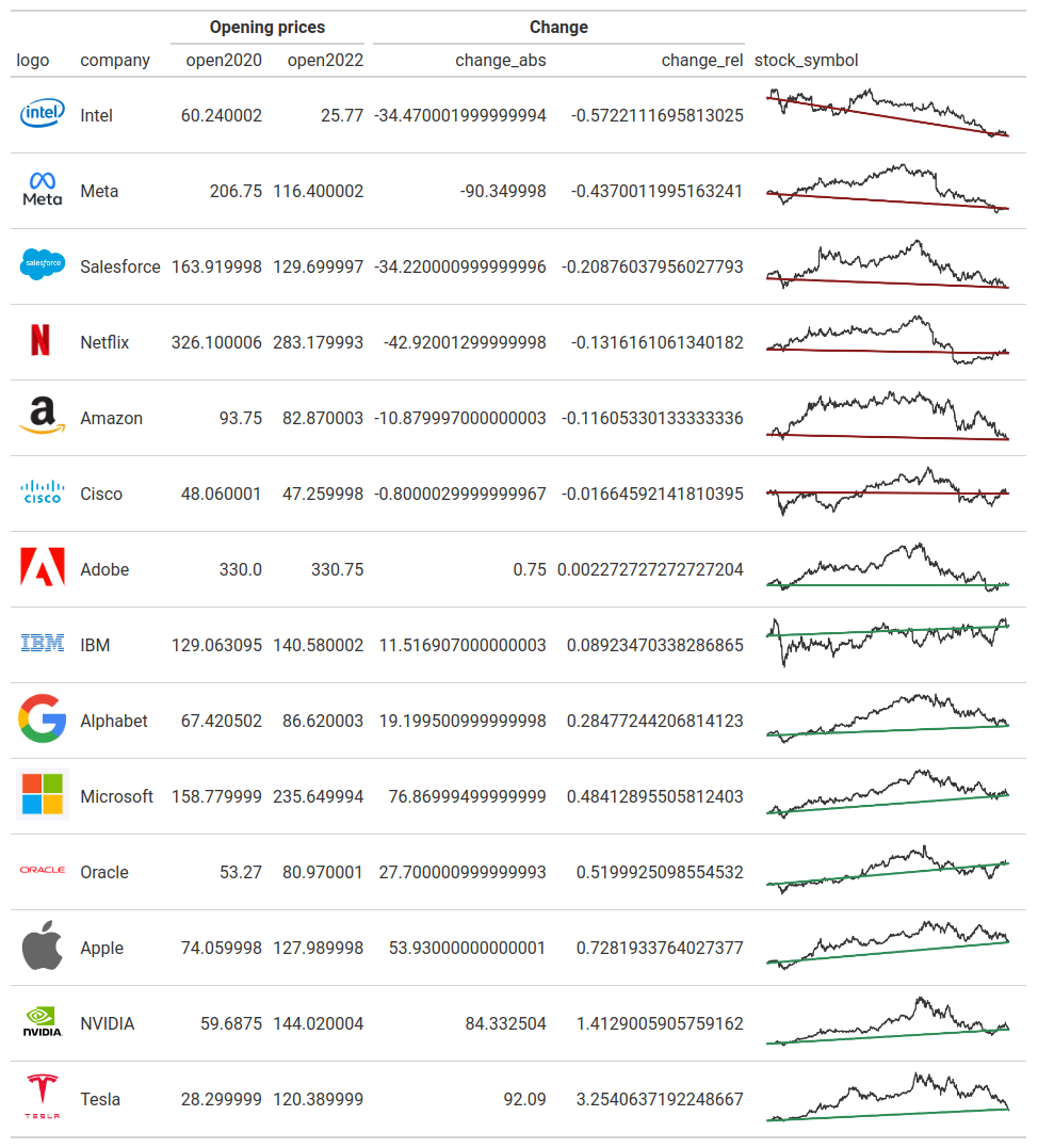
Nicely formatted numbers
So far so good. Let’s deal with the ugly numbers. Right now, nothing is formatted. We can change that with all of the fmt_*() functions that {gt} gives us. In particular, we can use fmt_currency() and fmt_percent() here.
library(gt)
gt(df_cleaned) |>
  fmt_markdown(
    columns = c(logo, stock_symbol)
  ) |>
  tab_spanner(
    label = md('**Opening prices**'),
    columns = c(open2020, open2022)
  ) |>
  tab_spanner(
    label = md('**Change**'),
    columns = c(change_abs, change_rel)
  ) |>
  cols_label(
    stock_symbol = md('**Opening prices over time**'),
    company = '',
    logo = '',
    open2020 = 'Jan 02, 2020',
    open2022 = 'Dec 29, 2022',
    change_abs = 'abs.',
    change_rel = 'rel.'
  ) |>
  fmt_currency(columns = c(open2020, open2022, change_abs)) |>
  fmt_percent(columns = change_rel)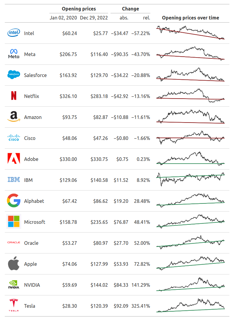
import great_tables as gt
(
  gt.GT(df_cleaned)
  .tab_spanner(
    label = gt.md('**Opening prices**'),
    columns = ["open2020", "open2022"]
  )
  .tab_spanner(
    label = gt.md('**Change**'),
    columns = ["change_abs", "change_rel"]
  )
  .cols_label(
    stock_symbol = gt.md('**Opening prices over time**'),
    company = '',
    logo = '',
    open2020 = 'Jan 02, 2020',
    open2022 = 'Dec 29, 2022',
    change_abs = 'abs.',
    change_rel = 'rel.'
  )
  .fmt_currency(columns = ["open2020", "open2022", "change_abs"])
  .fmt_percent(columns = "change_rel")
)
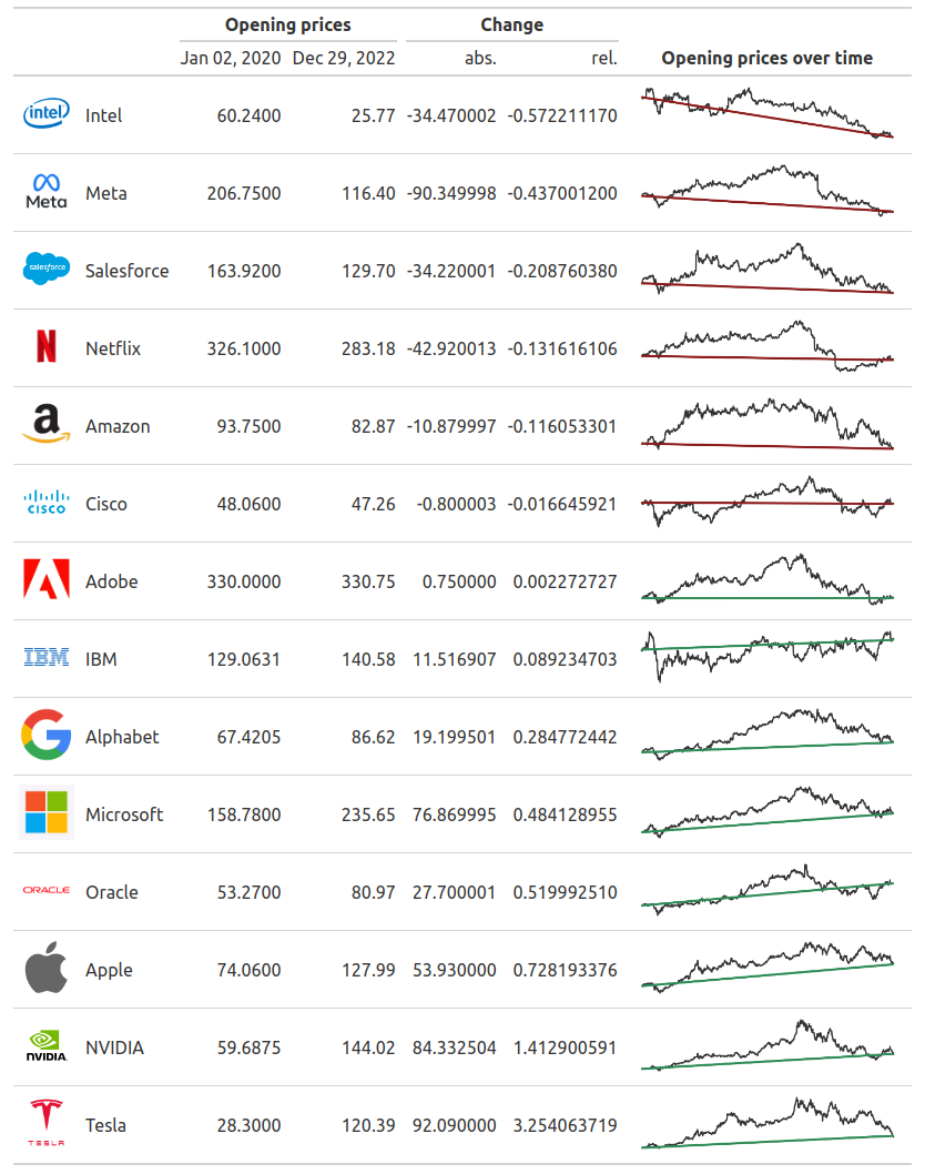
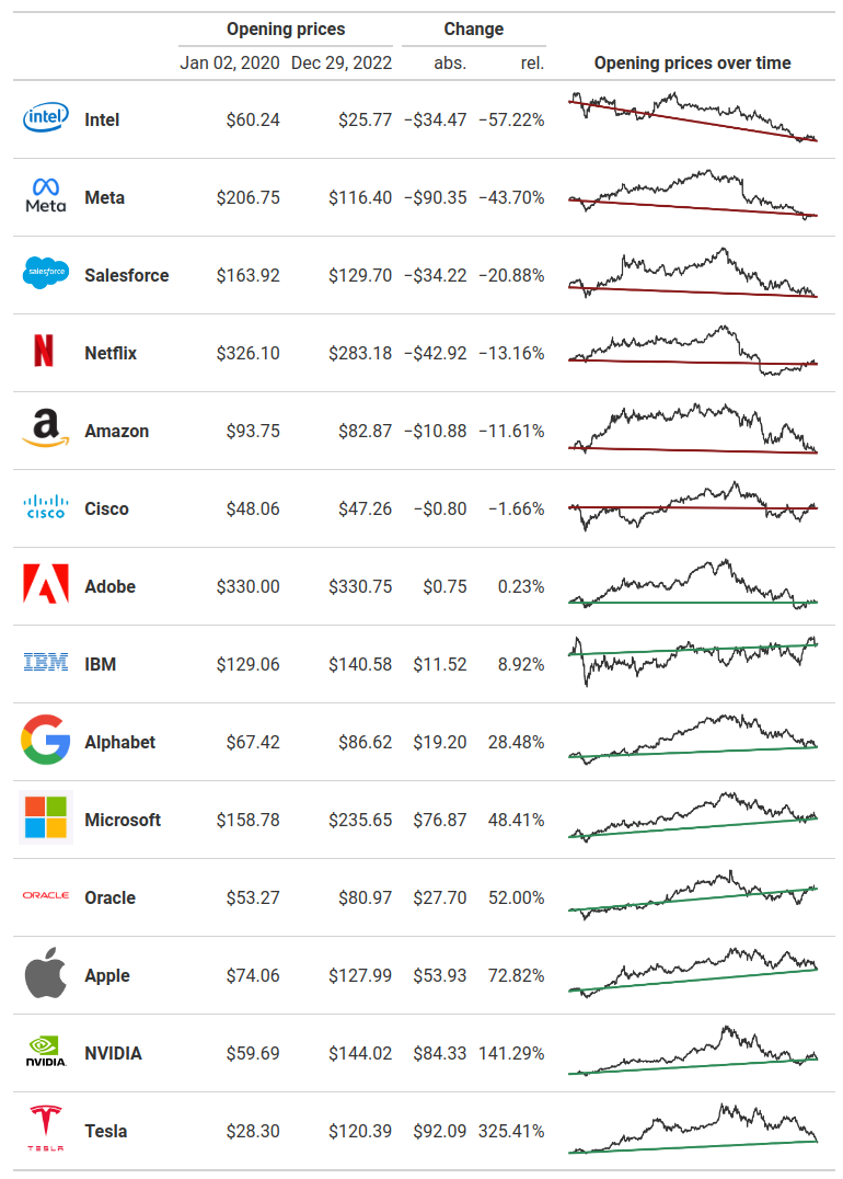
Align columns
We’re getting closer to our final image. Next, let us talk about aligning columns. Typically, you want numbers to be right-aligned and texts to be left-aligned. Thankfully, {gt} does all of that for us automatically. But we might want to have the line charts center-aligned. We can change any column alignment with cols_align().
library(gt)
gt(df_cleaned) |>
fmt_markdown(
columns = c(logo, stock_symbol)
) |>
tab_spanner(
label = md('**Opening prices**'),
columns = c(open2020, open2022)
) |>
tab_spanner(
label = md('**Change**'),
columns = c(change_abs, change_rel)
) |>
cols_label(
stock_symbol = md('**Opening prices over time**'),
company = '',
logo = '',
open2020 = 'Jan 02, 2020',
open2022 = 'Dec 29, 2022',
change_abs = 'abs.',
change_rel = 'rel.'
) |>
fmt_currency(columns = c(open2020, open2022, change_abs)) |>
fmt_percent(columns = change_rel) |>
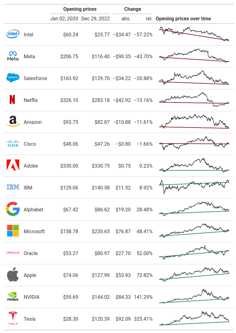
cols_align(columns = stock_symbol, align = 'center')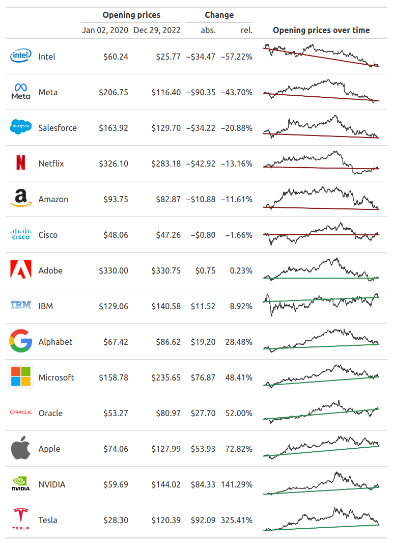
import great_tables as gt
(
  gt.GT(df_cleaned)
  .tab_spanner(
    label = gt.md('**Opening prices**'),
    columns = ["open2020", "open2022"]
  )
  .tab_spanner(
    label = gt.md('**Change**'),
    columns = ["change_abs", "change_rel"]
  )
  .cols_label(
    stock_symbol = gt.md('**Opening prices over time**'),
    company = '',
    logo = '',
    open2020 = 'Jan 02, 2020',
    open2022 = 'Dec 29, 2022',
    change_abs = 'abs.',
    change_rel = 'rel.'
  )
  .fmt_currency(columns = ["open2020", "open2022", "change_abs"])
  .fmt_percent(columns = "change_rel")
  .cols_align(columns = 'stock_symbol', align = 'center')
)
Formatting texts
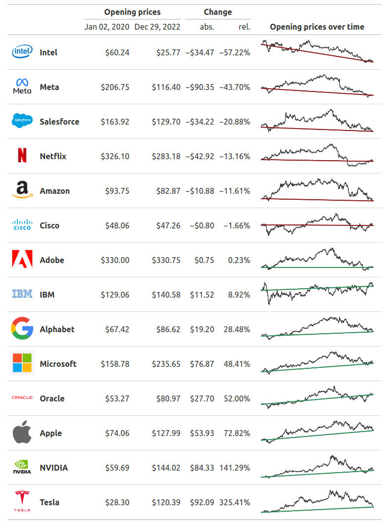
Now, let’s move a bit into the text styling. For example, you might want to modify the appearance of the text in the column that displays the company names. That’s where the function tab_style() comes in. It helps us to change the style of a table cell.
The trick is to use a helper function that selects the right cells that we want to style differently. For that, R has cells_body() and Python has loc.body(). And just like there is a helper function to select the targeted cells, there’s a function to help you with defining the style. In R that’s cell_text() and in Python you can use style.text().
library(gt)
gt(df_cleaned) |>
  fmt_markdown(
    columns = c(logo, stock_symbol)
  ) |>
  tab_spanner(
    label = md('**Opening prices**'),
    columns = c(open2020, open2022)
  ) |>
  tab_spanner(
    label = md('**Change**'),
    columns = c(change_abs, change_rel)
  ) |>
  cols_label(
    stock_symbol = md('**Opening prices over time**'),
    company = '',
    logo = '',
    open2020 = 'Jan 02, 2020',
    open2022 = 'Dec 29, 2022',
    change_abs = 'abs.',
    change_rel = 'rel.'
  ) |>
  fmt_currency(columns = c(open2020, open2022, change_abs)) |>
  fmt_percent(columns = change_rel) |>
  cols_align(columns = stock_symbol, align = 'center') |>
  tab_style(
    style = cell_text(weight = 'bold'),
    locations = cells_body(columns = company)
  )
import great_tables as gt
(
  gt.GT(df_cleaned)
  .tab_spanner(
    label = gt.md('**Opening prices**'),
    columns = ["open2020", "open2022"]
  )
  .tab_spanner(
    label = gt.md('**Change**'),
    columns = ["change_abs", "change_rel"]
  )
  .cols_label(
    stock_symbol = gt.md('**Opening prices over time**'),
    company = '',
    logo = '',
    open2020 = 'Jan 02, 2020',
    open2022 = 'Dec 29, 2022',
    change_abs = 'abs.',
    change_rel = 'rel.'
  )
  .fmt_currency(columns = ["open2020", "open2022", "change_abs"])
  .fmt_percent(columns = "change_rel")
  .cols_align(columns = 'stock_symbol', align = 'center')
  .tab_style(
    style = gt.style.text(weight = 'bold'),
    locations = gt.loc.body(columns = 'company')
  )
)
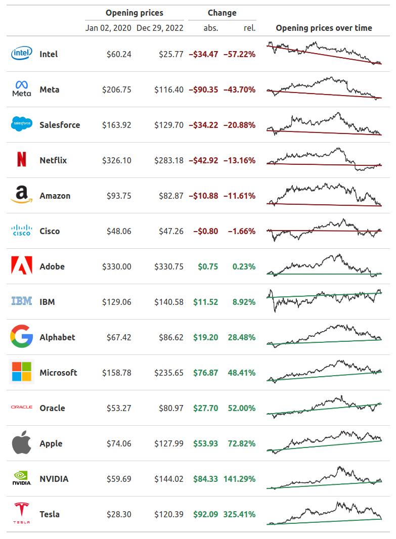
Conditional formatting
As you can see in the final image, the “Change” columns have a conditional formatting. This means that they use red text when the numbers are negative and green text when the numbers are positive. Once again, we can achieve that with tab_style().
Here, the trick is to target the right rows in the table body. Luckily, both cells_body() in R and loc.body() understand expressions for selecting the right rows based on the data values. That’s a pretty neat feature for conditional formatting.
library(gt)
gt(df_cleaned) |>
  fmt_markdown(
    columns = c(logo, stock_symbol)
  ) |>
  tab_spanner(
    label = md('**Opening prices**'),
    columns = c(open2020, open2022)
  ) |>
  tab_spanner(
    label = md('**Change**'),
    columns = c(change_abs, change_rel)
  ) |>
  cols_label(
    stock_symbol = md('**Opening prices over time**'),
    company = '',
    logo = '',
    open2020 = 'Jan 02, 2020',
    open2022 = 'Dec 29, 2022',
    change_abs = 'abs.',
    change_rel = 'rel.'
  ) |>
  fmt_currency(columns = c(open2020, open2022, change_abs)) |>
  fmt_percent(columns = change_rel) |>
  cols_align(columns = stock_symbol, align = 'center') |>
  tab_style(
    style = cell_text(weight = 'bold'),
    locations = cells_body(columns = company)
  ) |>
  # Style negative values
  tab_style(
    style = cell_text(color = '#8b1a1a', weight = 'bold'),
    locations = cells_body(
        columns = c(change_abs, change_rel),
        rows =  (change_abs < 0)
    )
  ) |>
  # Style non-negative values
  tab_style(
    style = cell_text(color = '#2E8B57', weight = 'bold'),
    locations = cells_body(
        columns = c(change_abs, change_rel),
        rows =  (change_abs >= 0)
    )
  )
import great_tables as gt
(
  gt.GT(df_cleaned)
  .tab_spanner(
    label = gt.md('**Opening prices**'),
    columns = ["open2020", "open2022"]
  )
  .tab_spanner(
    label = gt.md('**Change**'),
    columns = ["change_abs", "change_rel"]
  )
  .cols_label(
    stock_symbol = gt.md('**Opening prices over time**'),
    company = '',
    logo = '',
    open2020 = 'Jan 02, 2020',
    open2022 = 'Dec 29, 2022',
    change_abs = 'abs.',
    change_rel = 'rel.'
  )
  .fmt_currency(columns = ["open2020", "open2022", "change_abs"])
  .fmt_percent(columns = "change_rel")
  .cols_align(columns = 'stock_symbol', align = 'center')
  .tab_style(
    style = gt.style.text(weight = 'bold'),
    locations = gt.loc.body(columns = 'company')
  )
  # Style negative values
  .tab_style(
    style = gt.style.text(color = '#8b1a1a', weight = 'bold'),
    locations = gt.loc.body(
        columns = ["change_abs", "change_rel"] ,
        rows =  (pl.col("change_abs") < 0)
    )
  )
  # Style non-negative values
  .tab_style(
    style = gt.style.text(color = '#2E8B57', weight = 'bold'),
    locations = gt.loc.body(
        columns = ["change_abs", "change_rel"] ,
        rows =  (pl.col("change_abs") >= 0)
    )
  )
)
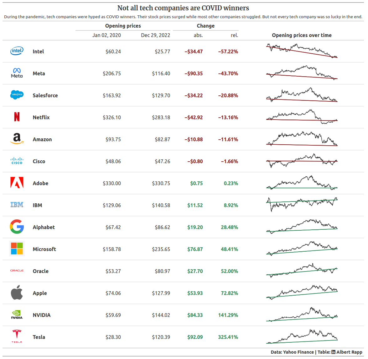
Add context with headlines, subtitles and source notes
Niiiiice! Our table is almost finished. But what we still need is more context that we get with headlines, subtitles and source notes. We can add those things with tab_header() and tab_source_note().
And as you can see in the final images, I want to use a different font for the headline and a LinkedIn icon in the source note. For the headline, there is an in-built feature in R to target the style of the headline. But it seems that this feature is not yet available in the Python version. But no problem. We can help ourselves with a bit us custom HTML & CSS.
Remember how we used the <img> tag and markdown formatting to display the images? We can do a similar thing for switching font families. That’s what the <span> tag is for. This tag produces nothing but inline text (that we have anyway) but we can use it to set the style attribute for custom stylings. Here, we use that for setting the font family of the headline and using the Font Awesome font for the LinkedIn icon.
library(gt)
gt(df_cleaned) |>
  fmt_markdown(
    columns = c(logo, stock_symbol)
  ) |>
  tab_spanner(
    label = md('**Opening prices**'),
    columns = c(open2020, open2022)
  ) |>
  tab_spanner(
    label = md('**Change**'),
    columns = c(change_abs, change_rel)
  ) |>
  cols_label(
    stock_symbol = md('**Opening prices over time**'),
    company = '',
    logo = '',
    open2020 = 'Jan 02, 2020',
    open2022 = 'Dec 29, 2022',
    change_abs = 'abs.',
    change_rel = 'rel.'
  ) |>
  fmt_currency(columns = c(open2020, open2022, change_abs)) |>
  fmt_percent(columns = change_rel) |>
  cols_align(columns = stock_symbol, align = 'center') |>
  tab_style(
    style = cell_text(weight = 'bold'),
    locations = cells_body(columns = company)
  ) |>
  tab_style(
    style = cell_text(color = '#8b1a1a', weight = 'bold'),
    locations = cells_body(
        columns = c(change_abs, change_rel),
        rows =  (change_abs < 0)
    )
  ) |>
  tab_style(
    style = cell_text(color = '#2E8B57', weight = 'bold'),
    locations = cells_body(
        columns = c(change_abs, change_rel),
        rows =  (change_abs >= 0)
    )
  ) |>
  tab_header(
    # Use markdown for span-tags
    title = md('<span style="font-family:Merriweather;">**Not all tech companies are COVID winners**</span>'),
    subtitle = 'During the pandemic, tech companies were hyped as COVID winners. Their stock prices surged while most other companies struggled. But not every tech company was so lucky in the end.'
  ) |>
  # Use span tags for Font Awesome
  # Use div for right-aligning and bold text
  tab_source_note(
    md("<div style='text-align:right; font-weight: 600;'>Data: Yahoo Finance | Table: <span style='font-family: \"Font Awesome 6 Brands\";'>linkedin</span> Albert Rapp</div>")
  )
import great_tables as gt
(
  gt.GT(df_cleaned)
  .tab_spanner(
    label = gt.md('**Opening prices**'),
    columns = ["open2020", "open2022"]
  )
  .tab_spanner(
    label = gt.md('**Change**'),
    columns = ["change_abs", "change_rel"]
  )
  .cols_label(
    stock_symbol = gt.md('**Opening prices over time**'),
    company = '',
    logo = '',
    open2020 = 'Jan 02, 2020',
    open2022 = 'Dec 29, 2022',
    change_abs = 'abs.',
    change_rel = 'rel.'
  )
  .fmt_currency(columns = ["open2020", "open2022", "change_abs"])
  .fmt_percent(columns = "change_rel")
  .cols_align(columns = 'stock_symbol', align = 'center')
  .tab_style(
    style = gt.style.text(weight = 'bold'),
    locations = gt.loc.body(columns = 'company')
  )
  .tab_style(
    style = gt.style.text(color = '#8b1a1a', weight = 'bold'),
    locations = gt.loc.body(
        columns = ["change_abs", "change_rel"] ,
        rows =  (pl.col("change_abs") < 0)
    )
  )
  .tab_style(
    style = gt.style.text(color = '#2E8B57', weight = 'bold'),
    locations = gt.loc.body(
        columns = ["change_abs", "change_rel"] ,
        rows =  (pl.col("change_abs") >= 0)
    )
  )
  .tab_header(
    # Use markdown for span-tags
    title = gt.md('<span style="font-family:Merriweather;">**Not all tech companies are COVID winners**</span>'),
    subtitle = 'During the pandemic, tech companies were hyped as COVID winners. Their stock prices surged while most other companies struggled. But not every tech company was so lucky in the end.'
  )
  .tab_source_note(
    # Use span tags for Font Awesome
    # Use div for right-aligning and bold text
    source_note = gt.md("<div style='text-align:right; font-weight: 600;'>Data: Yahoo Finance | Table: <span style='font-family: \"Font Awesome 6 Brands\";'>linkedin</span> Albert Rapp</div>")
  )
)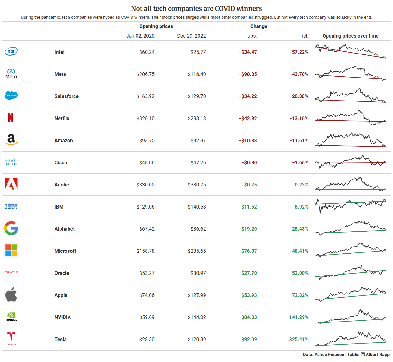
Finishing touches with table-wide settings
Excellent! We’re almost done. We can add finishing touches by changing a few general table settings. All of these get funneled through tab_options().
library(gt)
gt(df_cleaned) |>
  fmt_markdown(
    columns = c(logo, stock_symbol)
  ) |>
  tab_spanner(
    label = md('**Opening prices**'),
    columns = c(open2020, open2022)
  ) |>
  tab_spanner(
    label = md('**Change**'),
    columns = c(change_abs, change_rel)
  ) |>
  cols_label(
    stock_symbol = md('**Opening prices over time**'),
    company = '',
    logo = '',
    open2020 = 'Jan 02, 2020',
    open2022 = 'Dec 29, 2022',
    change_abs = 'abs.',
    change_rel = 'rel.'
  ) |>
  fmt_currency(columns = c(open2020, open2022, change_abs)) |>
  fmt_percent(columns = change_rel) |>
  cols_align(columns = stock_symbol, align = 'center') |>
  tab_style(
    style = cell_text(weight = 'bold'),
    locations = cells_body(columns = company)
  ) |>
  tab_style(
    style = cell_text(color = '#8b1a1a', weight = 'bold'),
    locations = cells_body(
        columns = c(change_abs, change_rel),
        rows =  (change_abs < 0)
    )
  ) |>
  tab_style(
    style = cell_text(color = '#2E8B57', weight = 'bold'),
    locations = cells_body(
        columns = c(change_abs, change_rel),
        rows =  (change_abs >= 0)
    )
  ) |>
  tab_header(
    title = md('<span style="font-family:Merriweather;">**Not all tech companies are COVID winners**</span>'),
    subtitle = 'During the pandemic, tech companies were hyped as COVID winners. Their stock prices surged while most other companies struggled. But not every tech company was so lucky in the end.'
  ) |>
  tab_source_note(
    md("<div style='text-align:right; font-weight: 600;'>Data: Yahoo Finance | Table: <span style='font-family: \"Font Awesome 6 Brands\";'>linkedin</span> Albert Rapp</div>")
  ) |>
  tab_options(
    heading.title.font.size = '40px',
    heading.subtitle.font.size= '24px',
    heading.align = 'left',
    table.font.names = 'Source Sans Pro' ,
    container.width='900px'
  )
import great_tables as gt
(
  gt.GT(df_cleaned)
  .tab_spanner(
    label = gt.md('**Opening prices**'),
    columns = ["open2020", "open2022"]
  )
  .tab_spanner(
    label = gt.md('**Change**'),
    columns = ["change_abs", "change_rel"]
  )
  .cols_label(
    stock_symbol = gt.md('**Opening prices over time**'),
    company = '',
    logo = '',
    open2020 = 'Jan 02, 2020',
    open2022 = 'Dec 29, 2022',
    change_abs = 'abs.',
    change_rel = 'rel.'
  )
  .fmt_currency(columns = ["open2020", "open2022", "change_abs"])
  .fmt_percent(columns = "change_rel")
  .cols_align(columns = 'stock_symbol', align = 'center')
  .tab_style(
    style = gt.style.text(weight = 'bold'),
    locations = gt.loc.body(columns = 'company')
  )
  .tab_style(
    style = gt.style.text(color = '#8b1a1a', weight = 'bold'),
    locations = gt.loc.body(
        columns = ["change_abs", "change_rel"] ,
        rows =  (pl.col("change_abs") < 0)
    )
  )
  .tab_style(
    style = gt.style.text(color = '#2E8B57', weight = 'bold'),
    locations = gt.loc.body(
        columns = ["change_abs", "change_rel"] ,
        rows =  (pl.col("change_abs") >= 0)
    )
  )
  .tab_header(
    title = gt.md('<span style="font-family:Merriweather;">**Not all tech companies are COVID winners**</span>'),
    subtitle = 'During the pandemic, tech companies were hyped as COVID winners. Their stock prices surged while most other companies struggled. But not every tech company was so lucky in the end.'
  )
  .tab_source_note(
    source_note = gt.md("<div style='text-align:right; font-weight: 600;'>Data: Yahoo Finance | Table: <span style='font-family: \"Font Awesome 6 Brands\";'>linkedin</span> Albert Rapp</div>")
  )
  .tab_options(
      heading_title_font_size = '40px',
      heading_subtitle_font_size= '24px',
      heading_align = 'left',
      table_font_names = 'Source Sans Pro' ,
      container_width ='900px'
  )
)
Conclusion
BAAAM! We made it. That was quite a long ride. But I like to think this was worth it. We created two nice tables with the gt package. In both R and Python, mind you! That’s no small feat to accomplish. And all of that was the result of the excellent work of the Posit dev team.
I hope y’all enjoyed the blog post. Have a great day and see you next time. And if you found this helpful, here are some other ways I can help you:
- 3 Minute Wednesdays: A weekly newsletter with bite-sized tips and tricks for R users
- Insightful Data Visualizations for “Uncreative” R Users: A course that teaches you how to leverage
{ggplot2}to make charts that communicate effectively without being a design expert.


