Three Ways to Include Images in Your ggplots

Visualization

In this blog post, I show you three ways to include image files into your ggplot2 plots

Author

Albert Rapp

Published

April 7, 2024

In today’s blog post, I want to show you how you can use images in your ggplots. I will show you three ways for three different use cases. And as always, you can find the video version of this blog post on Youtube:

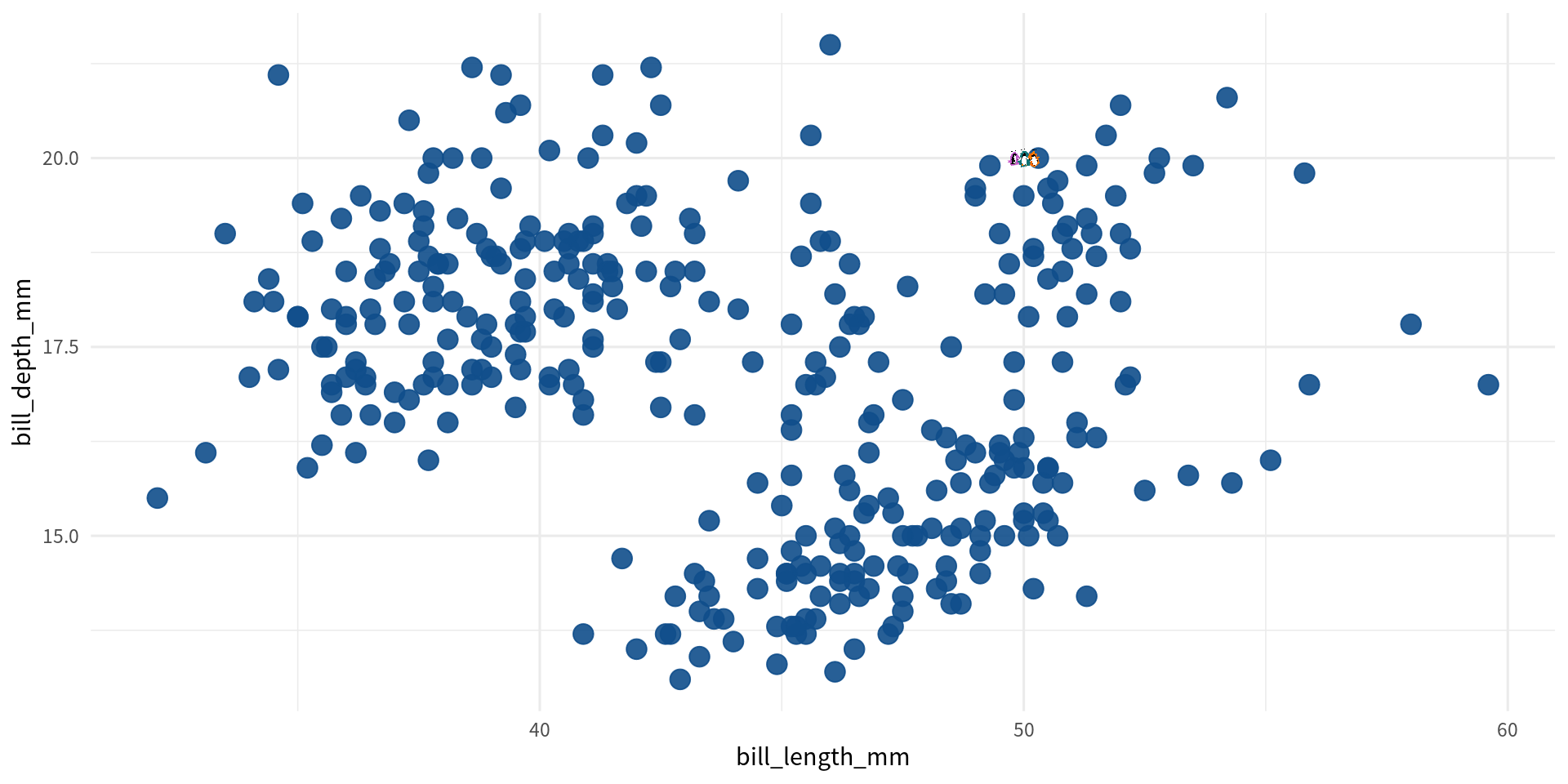
Using images inside the main panel with `geom_image()`

The first way to add images is the easiest. You can use any image inside your plot’s main panel using the geom_image() function from the ggimage package. So let’s say you have the following scatter plot:

library(tidyverse)
palmerpenguins::penguins |> 
  ggplot(aes(x = bill_length_mm, y = bill_depth_mm)) +
  geom_point(size = 4, color = 'dodgerblue4', alpha = 0.9) +
  theme_minimal(
    base_size = 12,
    base_family = 'Source Sans Pro'
  )

And now you want to add the following delightful image by Allison Horst to your plot:

You can do this by loading the ggimage package and adding a geom_image() layer to it. There, you will have to map the image aesthetic to that image file (that you should have downloaded at this point). Make sure that the data argument is a single-row data set, otherwise it will add the image multiple times.

library(ggimage)
palmerpenguins::penguins |> 
  ggplot(aes(x = bill_length_mm, y = bill_depth_mm)) +
  geom_point(size = 4, color = 'dodgerblue4', alpha = 0.9)+
  theme_minimal(
    base_size = 12,
    base_family = 'Source Sans Pro'
  ) +
  geom_image(
    data = tibble(bill_length_mm = 50, bill_depth_mm = 20),
    aes(image = "penguins.png")
  )

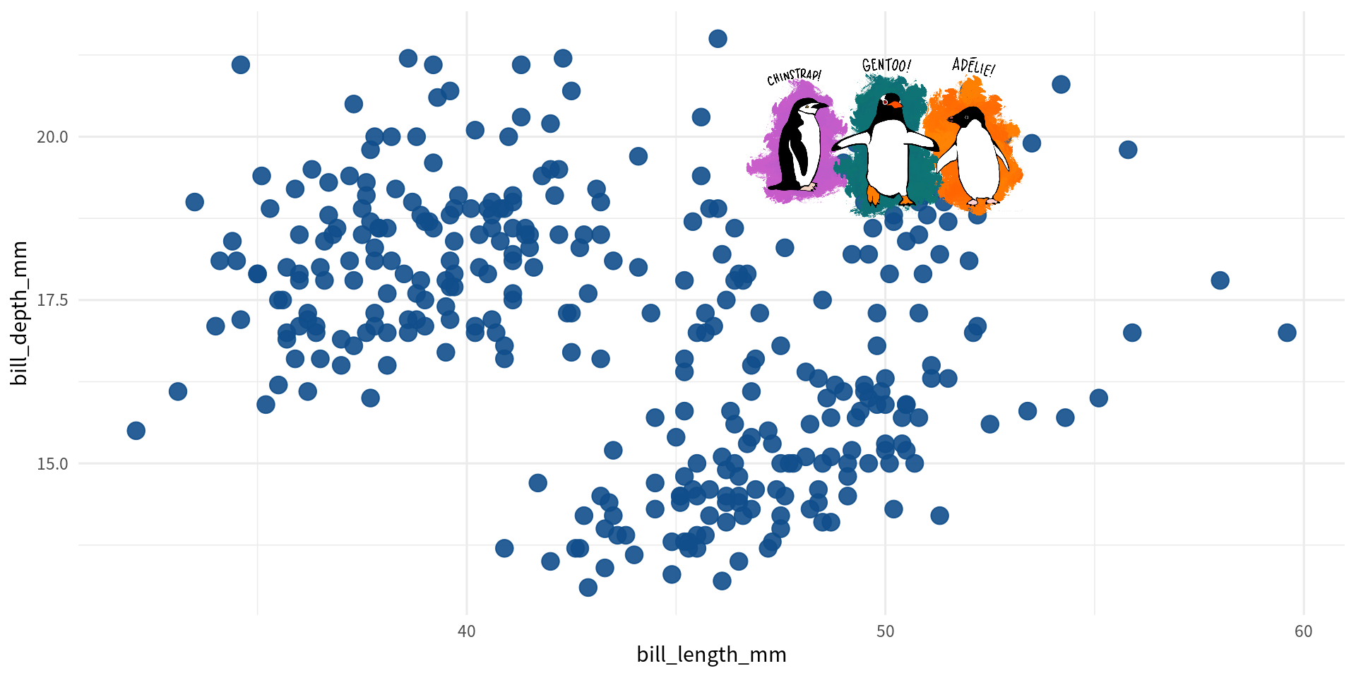
With the size argument, you can then adjust the size of the image.

palmerpenguins::penguins |> 
  ggplot(aes(x = bill_length_mm, y = bill_depth_mm)) +
  geom_point(size = 4, color = 'dodgerblue4', alpha = 0.9)+
  theme_minimal(
    base_size = 12,
    base_family = 'Source Sans Pro'
  ) +
  geom_image(
    data = tibble(bill_length_mm = 50, bill_depth_mm = 20),
    aes(image = "penguins.png"),
    size = 0.5
  )

Using images inside geoms

The second strategy is similar, but it uses images inside of geoms that you are already using. For example, imagine that you have a waffle chart like this:

tibble(id = 0:22, row = id %% 5, col = id %/% 5) |> 
  ggplot(aes(x = col, y = row)) +
  geom_tile(fill = 'dodgerblue4', col = 'white', linewidth = 1) +
  coord_equal() +
  labs(title = 'Random waffle') +
  theme_void(base_size = 18, base_family = 'Source Sans Pro')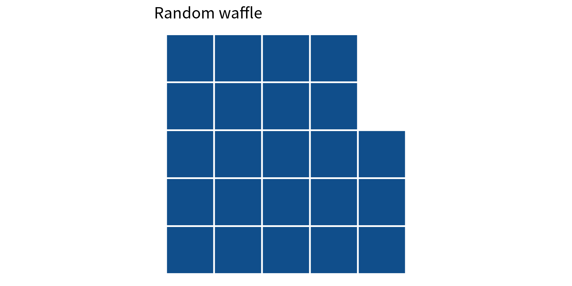

And now imagine that instead of the squares, we want to use an icon. This is where we’ll

use ggpattern,
replace geom_rect() with geom_rect_pattern(),
set the pattern to image, and
set the pattern_filename to the icon image you want to use.

This of course requires us to have the icon image downloaded and saved on our computer. For example, one of the icons from Flaticon will do. Assuming that we have downloaded and saved the image as sneaker.png, we can now use it in our waffle chart:

library(ggpattern)
tibble(id = 0:22, row = id %% 5, col = id %/% 5) |> 
  ggplot(aes(x = col, y = row)) +
  geom_tile_pattern(
    fill = 'dodgerblue4', 
    col = 'white', 
    linewidth = 1,
    pattern = 'image',
    pattern_filename = 'sneaker.png'
  ) +
  coord_equal() +
  labs(
    title = 'Random waffle',
    caption = 'Flaticon Icon by Us and Up'
  ) +
  theme_void(base_size = 18, base_family = 'Source Sans Pro')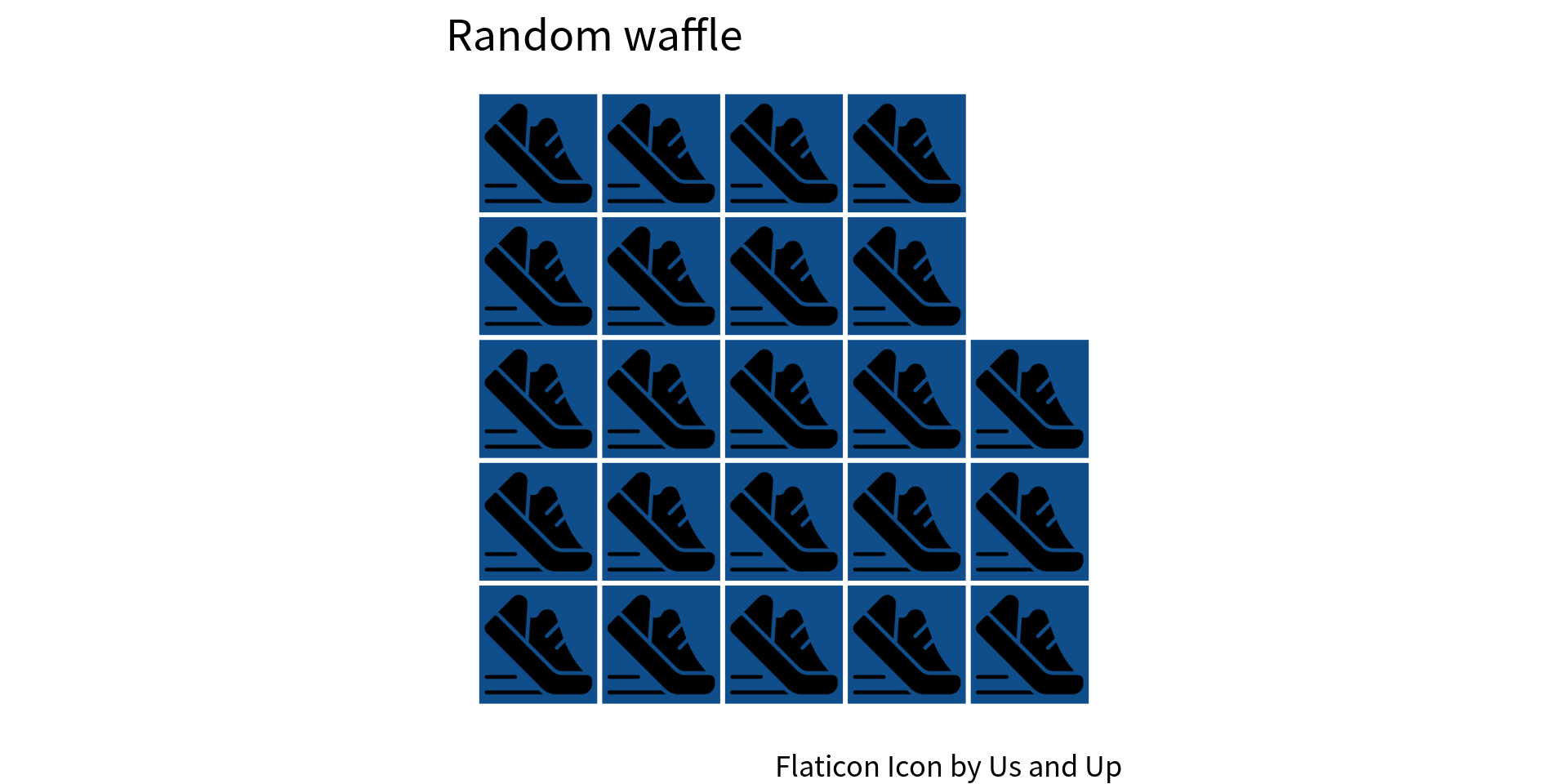

Notice how the sneakers are now inserted into the tiles. So instead of filling the squares blue we can make the background white.

tibble(id = 0:22, row = id %% 5, col = id %/% 5) |> 
  ggplot(aes(x = col, y = row)) +
  geom_tile_pattern(
    fill = 'white',  # Change here and remove col and linewidth
    pattern = 'image',
    pattern_filename = 'sneaker.png'
  ) +
  coord_equal() +
  labs(
    title = 'Random waffle',
    caption = 'Flaticon Icon by Us and Up'
  ) +
  theme_void(base_size = 18, base_family = 'Source Sans Pro')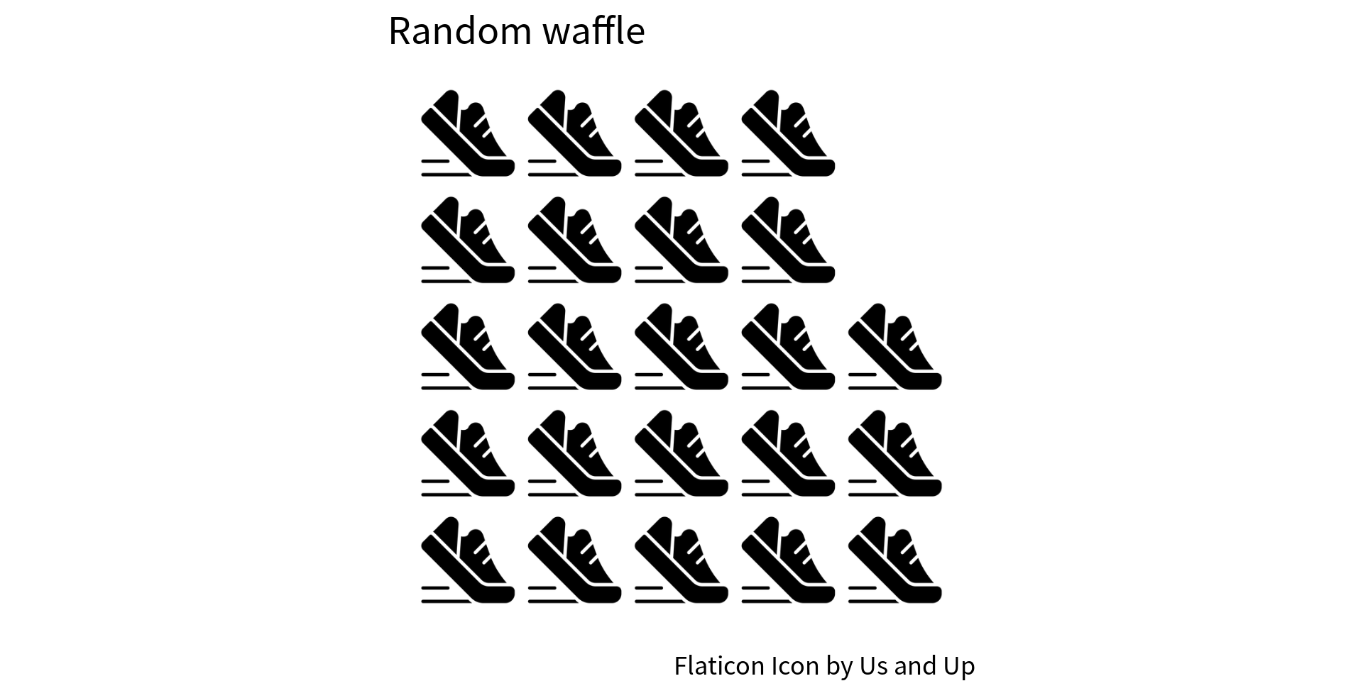

And you can specify a width and height to change the size of the icon.

tibble(id = 0:22, row = id %% 5, col = id %/% 5) |> 
  ggplot(aes(x = col, y = row)) +
  geom_tile_pattern(
    fill = 'white',  # Change here and remove col and linewidth
    pattern = 'image',
    pattern_filename = 'sneaker.png',
    width = 1.1,
    height = 1.1
  ) +
  coord_equal() +
  labs(
    title = 'Random waffle',
    caption = 'Flaticon Icon by Us and Up'
  ) +
  theme_void(base_size = 18, base_family = 'Source Sans Pro')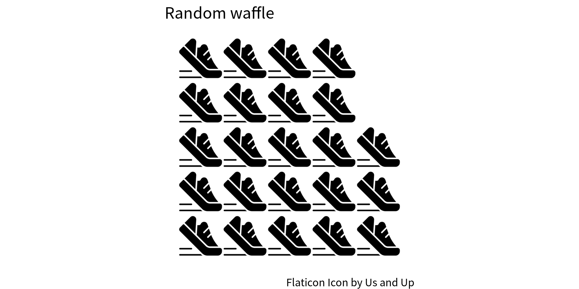

If you want to use differently colored versions of the icon, you can use the magick package to replace everything but the transparent bits with another color. Here’s how that works

library(magick)
raster <- image_read('sneaker.png') |> image_raster(tidy = FALSE)
raster[raster != "transparent"] <- 'dodgerblue4'
ragg::agg_png(
  'sneaker_blue.png', 512, 512, background = 'transparent'
)
plot(raster)  
dev.off()
## png 
##   2

That way, you have a new image file and can use it as part of the geom_rect_pattern() layer.

tibble(id = 0:22, row = id %% 5, col = id %/% 5) |> 
  ggplot(aes(x = col, y = row)) +
  geom_tile_pattern(
    fill = 'white',  # Change here and remove col and linewidth
    pattern = 'image',
    pattern_filename = 'sneaker_blue.png',
    width = 1.1,
    height = 1.1
  ) +
  coord_equal() +
  labs(
    title = 'Random waffle',
    caption = 'Flaticon Icon by Us and Up'
  ) +
  theme_void(base_size = 18, base_family = 'Source Sans Pro')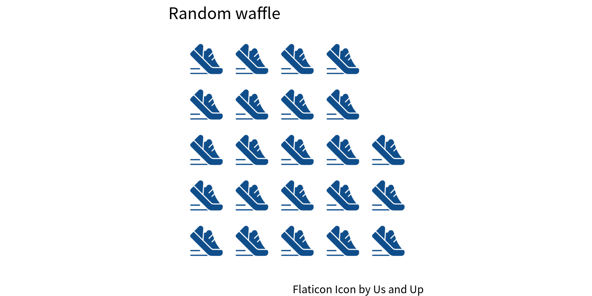

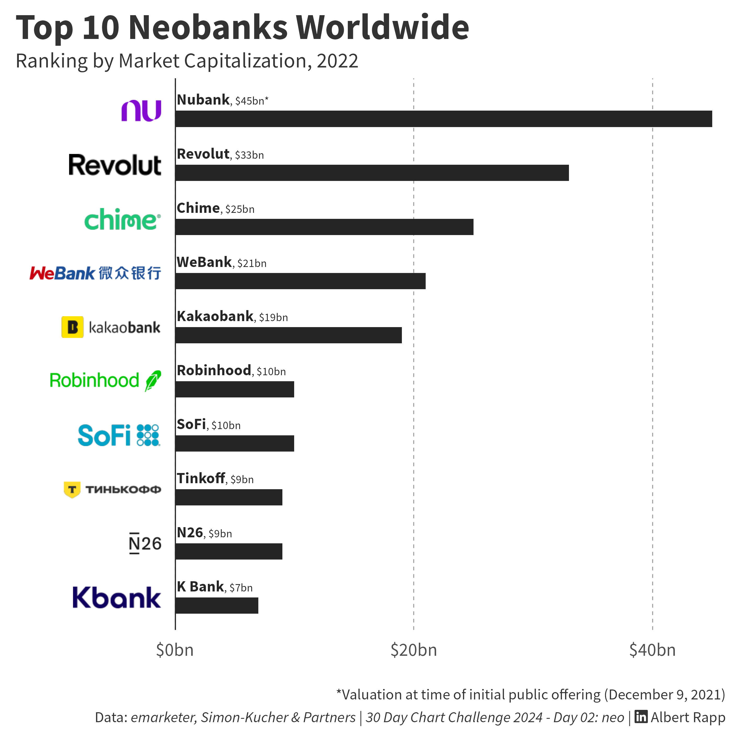
Using images as axis labels

The third trick requires a little bit of HTML and CSS notation. But it’s a good one. It allows you to use images as axis labels. For example, I’ve recently used this in the 30 Day Chart Challenge:

And to do that, you can use the ggtext package. Instead of regular labels, you can use <img> tags from HTML and CSS. All you have to do is to

replace the labels with something like <img src="file_for_label_replacement.png"> and
use this as labels for your axes.

But this requires you to have the png files on your computer or can find a url to the png file online. And for my recent contribution to the 30 Day Chart Challenge, I could only find svg images. Hence, I downloaded the svgs with magick and converted it to png. Here’s the code for that:

# market cat data from https://www.emarketer.com/chart/257463/top-10-neobanks-worldwide-by-market-capitalization-2022-billions
dat <- tribble(
  ~neo_bank, ~market_cap_bn, ~logo_url,
  "Nubank", 45, "https://upload.wikimedia.org/wikipedia/commons/f/f7/Nubank_logo_2021.svg",
  "Revolut", 33, "https://upload.wikimedia.org/wikipedia/commons/d/d6/Revolut.svg",
  "Chime", 25, "https://upload.wikimedia.org/wikipedia/commons/f/f6/Chime_company_logo.svg",
  "WeBank", 21, "https://upload.wikimedia.org/wikipedia/en/e/eb/WeBank_Logo.svg",
  "Kakaobank", 19, "https://upload.wikimedia.org/wikipedia/commons/4/48/KakaoBank_logo.svg",
  "Robinhood", 10, "https://upload.wikimedia.org/wikipedia/commons/d/da/Robinhood_%28company%29_logo.svg",
  "SoFi", 10, "https://upload.wikimedia.org/wikipedia/commons/1/16/SoFi_logo.svg",
  "Tinkoff", 9, "https://upload.wikimedia.org/wikipedia/commons/1/19/Tinkoff_logo_2024.svg",
  "N26", 9, "https://upload.wikimedia.org/wikipedia/commons/b/bf/N26_logo_2019.svg",
  "K Bank", 7, "https://upload.wikimedia.org/wikipedia/commons/2/26/Kbank_logo.svg"
) 
map(dat$logo_url, magick::image_read_svg) |>
  walk2(
    dat$neo_bank,
    \(x, y) magick::image_write(x, path = paste0("logos/", y, ".png"))
  )

This will save the images to a logos/ directory. And once you have those, you can use a combination of glue() and scale_y_discrete() to wrap the bank names into the <img> tags.

dat |> 
  mutate(neo_bank = fct_reorder(neo_bank, market_cap_bn)) |>
  ggplot(aes(x = market_cap_bn, y = neo_bank)) +
  geom_col() +
  scale_y_discrete(
    labels = \(x) glue::glue("<img src='logos/{x}.png' height=10 />")
  ) +
  theme_minimal(
    base_size = 12,
    base_family = 'Source Sans Pro'
  ) +
  labs(
    title = 'Top 10 neobanks worldwide by market capitalization 2022',
    y = element_blank()
  )

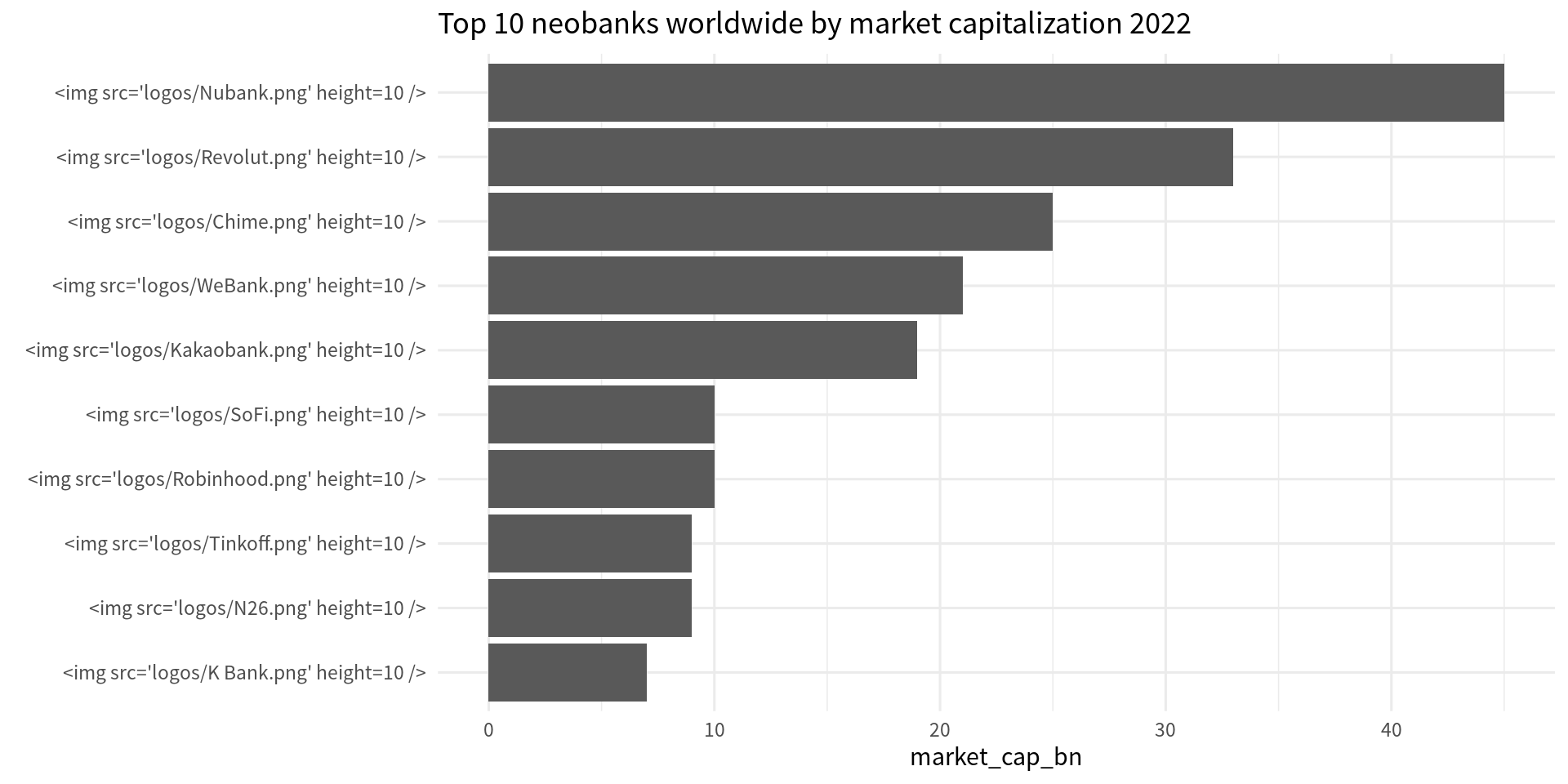
However, this will give you too much text on the axis rather than rendering this as image. The trick is to go into theme() and set the labels to element_markdown() from the ggtext package. This enables Markdown rendering and allows for HTML and CSS notation. This way, the <image> tag is turned into an actual image, and you have your image right where you want it to be.

dat |> 
  mutate(neo_bank = fct_reorder(neo_bank, market_cap_bn)) |>
  ggplot(aes(x = market_cap_bn, y = neo_bank))  +
  geom_col() +
  scale_y_discrete(
    labels = \(x) glue::glue("<img src='logos/{x}.png' height=20 />")
  ) +
  theme_minimal(
    base_size = 12,
    base_family = 'Source Sans Pro'
  ) +
  labs(
    title = 'Top 10 neobanks worldwide by market capitalization 2022',
    y = element_blank()
  ) +
  theme(
    axis.text.y = ggtext::element_markdown()
  )

Conclusion

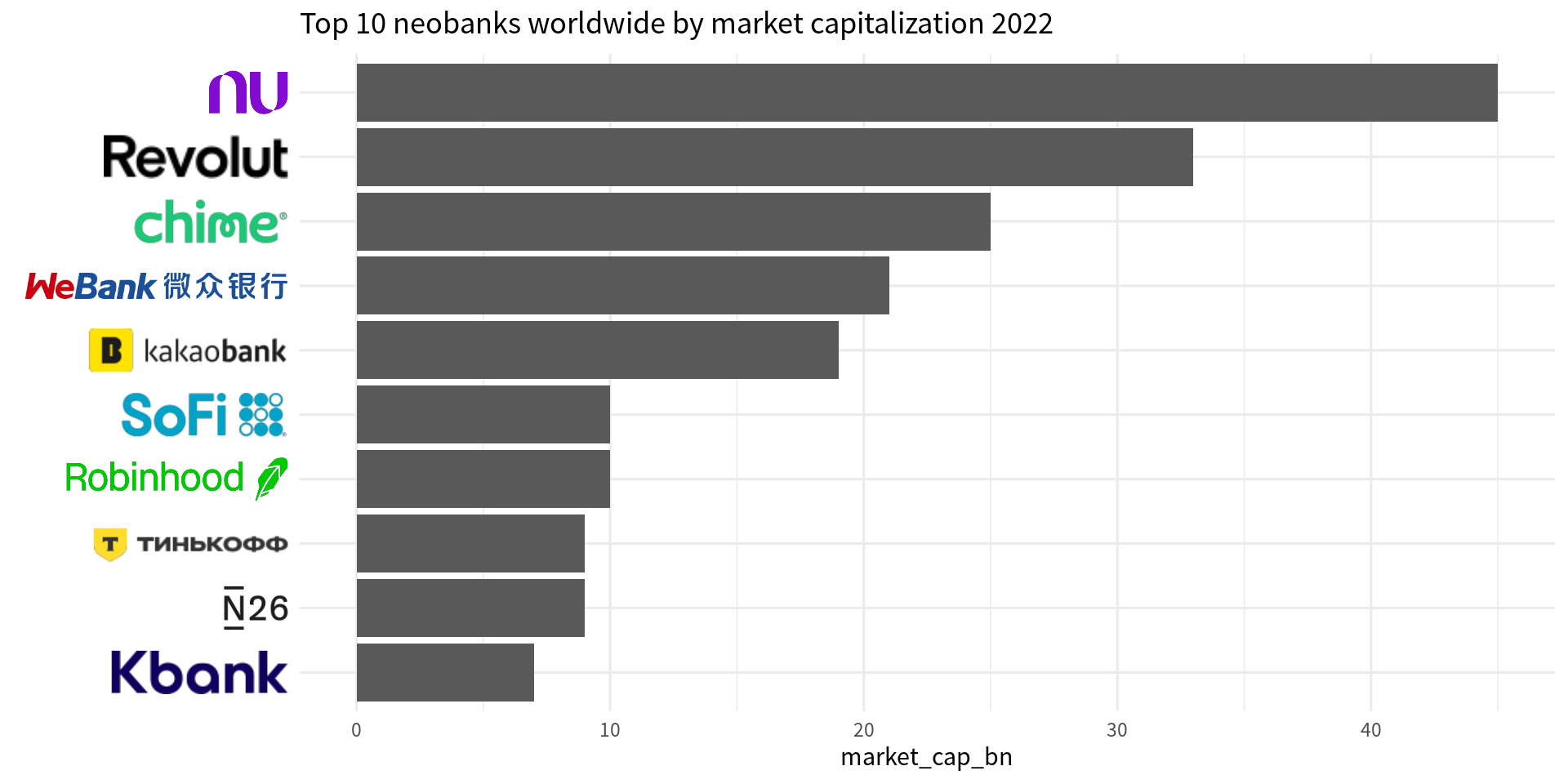
And there you have it! Three ways to use images inside your ggplots. Hope you enjoyed this little tutorial. Have a great day and see you next time. And if you found this helpful, here are some other ways I can help you:

3 Minute Wednesdays: A weekly newsletter with bite-sized tips and tricks for R users
Insightful Data Visualizations for “Uncreative” R Users: A course that teaches you how to leverage {ggplot2} to make charts that communicate effectively without being a design expert.

Three Ways to Include Images in Your ggplots

Using images inside the main panel with `geom_image()`

Using images inside geoms

Using images as axis labels

Conclusion

Stay in touch

You can also support my work with a coffee

Using images inside the main panel with geom_image()

Using images inside geoms

Using images as axis labels

Conclusion

Stay in touch

You can also support my work with a coffee

Using images inside the main panel with `geom_image()`