Text Styling With ggplot2

Today I’m showing you ggplot techniques that give you full control over your texts. This includes dynamic text colors (depending on the background) and customizations using the brand-new marquee package.

In today’s blog post, we are figuring out how to fully control the text styling of the texts that we put into our ggplots. This means that we will learn

• how to dynamically adjust the text color depending on the background color, and
• how to use the extensive styling capabilities that the brand-new {marquee} package gives you.

Here, you will find all of the code chunks split into sections. For detailed explantions, check out the corresponding YT video:

Customize the text color based on the background color

library(tidyverse)
dat <- tibble(value = 1:5) |> 
  mutate(
    text_color = if_else(
      value <= 3,
      'black',
      'white'
    )
  ) 

dat |> 
  ggplot(aes(x = value, y = 1)) +
  geom_tile(
    aes(fill = value),
    width = 0.5, 
    height = 0.5,
    col = 'black'
  ) +
  geom_text(
    aes(label = value),
    color = dat$text_color,
    size = 8,
    fontface = 'bold',
    family = 'Source Sans Pro'
  ) +
  coord_fixed() +
  scale_fill_gradient(low = 'white', high = 'firebrick4') +
  theme_void() +
  theme(legend.position = 'none')

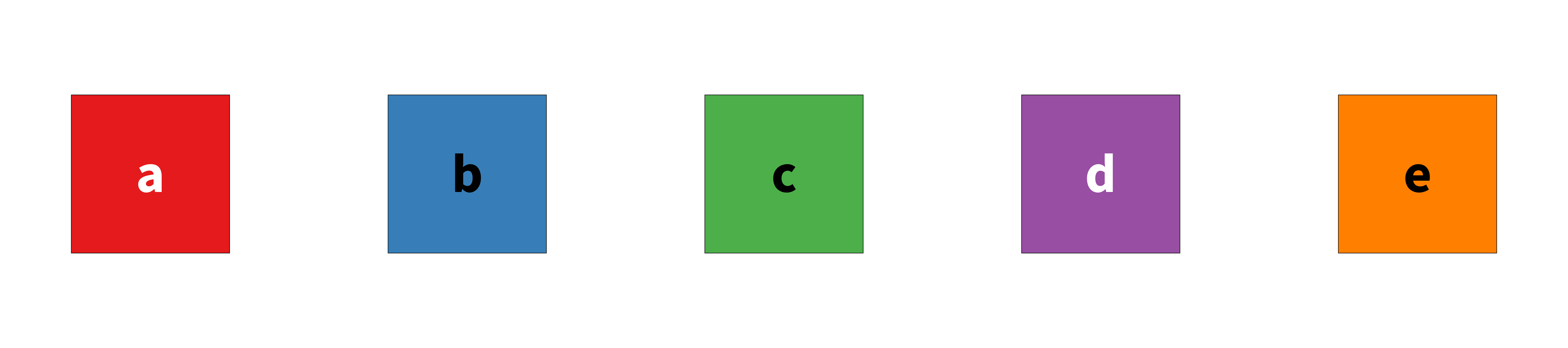
Dynamic text color with categorical labels

dat <- tibble(x = 1:5, letter = letters[1:5]) |> 
  mutate(
    text_color = if_else(
      letter %in% c('a', 'd'),
      'white',
      'black'
    )
  )

dat |> 
  ggplot(aes(x = x, y = 1)) +
  geom_tile(
    aes(fill = letter),
    width = 0.5, 
    height = 0.5,
    col = 'black'
  ) +
  geom_text(
    aes(label = letter),
    size = 8,
    color = dat$text_color,
    fontface = 'bold',
    family = 'Source Sans Pro'
  ) +
  coord_fixed() +
  theme_void() +
  scale_fill_brewer(palette = 'Set1') +
  theme(legend.position = 'none')

Use geom_marquee() instead of geom_text()

geom_marquee() is a drop-in replacement for geom_text() and geom_label(). Important caveat: In order for everything to render properly, you might have to update your ragg package

library(marquee)

md_text <- 'This is a **bold word** written in _Markdown_.'

tibble(x = 1, y = 1, label = md_text) |> 
  ggplot(aes(x, y)) +
  geom_marquee(
    aes(label = label),
    size = 13,
    family = 'Source Sans Pro'
  ) +
  theme_void()

Add more styles using the style aesthetic

tibble(x = 1, y = 1, label = md_text) |> 
  ggplot(aes(x, y)) +
  geom_marquee(
    aes(label = label),
    size = 13,
    family = 'Source Sans Pro',
    style = classic_style(
      weight = 'thin'
    )
  ) +
  theme_void()

Modify paragraph styles

my_own_style <- classic_style(
  weight = 'thin'
) |> 
  modify_style(
    'p', 
    background = 'dodgerblue4',
    padding = trbl(10),
    color = 'white',
    border_radius = 4
  )

tibble(x = 1, y = 1, label = md_text) |> 
  ggplot(aes(x, y)) +
  geom_marquee(
    aes(label = label),
    size = 13,
    family = 'Source Sans Pro',
    style = my_own_style
  ) +
  theme_void()

Modify Code styles

md_text <- 'Now let\'s try some `code` stuff and a [url]().'

tibble(x = 1, y = 1, label = md_text) |> 
  ggplot(aes(x, y)) +
  geom_marquee(
    aes(label = label),
    size = 13,
    family = 'Source Sans Pro',
    style = classic_style() |> 
      modify_style(
        'code',
        weight = 'bold',
        background = colorspace::lighten('dodgerblue4', 0.9),
        border_radius = 4,
        color = 'dodgerblue4',
        family = 'IBM Plex Mono',
        padding = trbl(0, 4, 0, 4)
      )
  ) +
  theme_void()

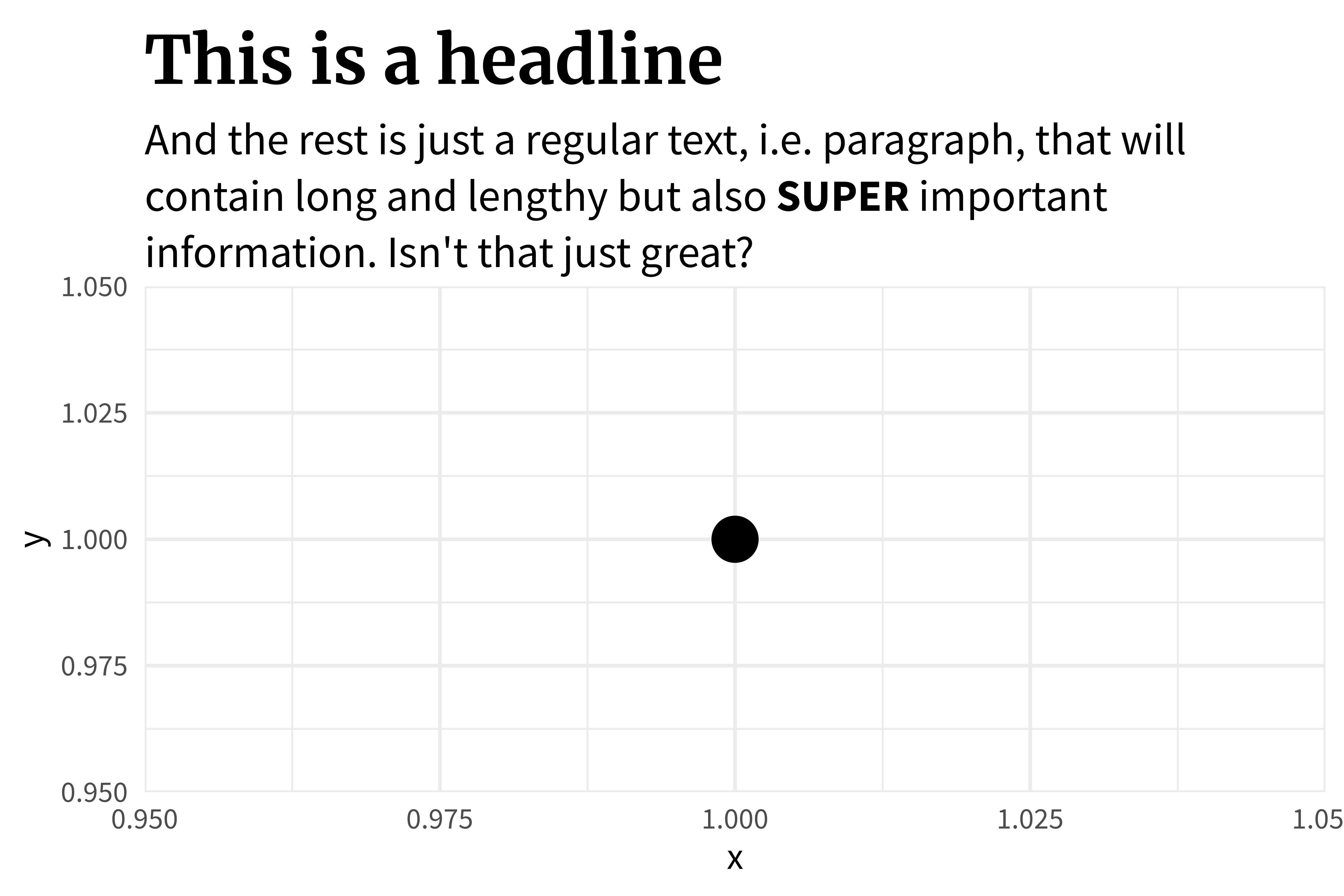
Use long texts as part of plot titles

md_text <- '# This is a headline

And the rest is just a regular text, i.e. paragraph, that will contain long and lengthy but also **SUPER** important information. Isn\'t that just great?'


headline_style <- classic_style() |> 
  remove_style('h1') |> 
  modify_style(
    'h1',
    weight = 'bold',
    size = 32,
    margin = trbl(b = 4),
    family = 'Merriweather'
  ) |> 
  modify_style(
    'p',
    lineheight = 1
  )

tibble(x = 1, y = 1) |> 
  ggplot(aes(x, y)) +
  geom_point(size = 10) +
  labs(title = md_text) +
  theme_minimal(
    base_size = 18, 
    base_family = 'Source Sans Pro'
  ) +
  theme(
    plot.title = element_marquee(
      width = 1,
      style = headline_style
    )
  )

Create text boxes using the width argument

text_box_style <- headline_style |> 
      modify_style(
        'p', 
        padding = trbl(l = 4),
        size = 16
      ) |> 
      modify_style(
        'body',
        border_radius = 4,
        border = 'dodgerblue4',
        border_size = trbl(2),
        padding = trbl(5)
      ) |> 
      modify_style(
        'h1',
        border_size = trbl(0)
      ) 

tibble(x = 1, y = 1) |> 
  ggplot(aes(x, y)) +
  geom_point(size = 10) +
  annotate(
    'marquee',
    x = 1.2,
    y = 1.5,
    label = md_text,
    width = 0.4,
    hjust = 0,
    fill = colorspace::lighten('dodgerblue1', 0.7),
    style = text_box_style
  ) +
  labs(title = md_text) +
  theme_minimal(
    base_size = 18, 
    base_family = 'Source Sans Pro'
  ) +
  theme(
    plot.title = element_marquee(
      width = 1,
      style = headline_style
    )
  ) +
  coord_cartesian(
    xlim = c(0, 2),
    ylim = c(0, 2)
  )

Colorize single words in your title

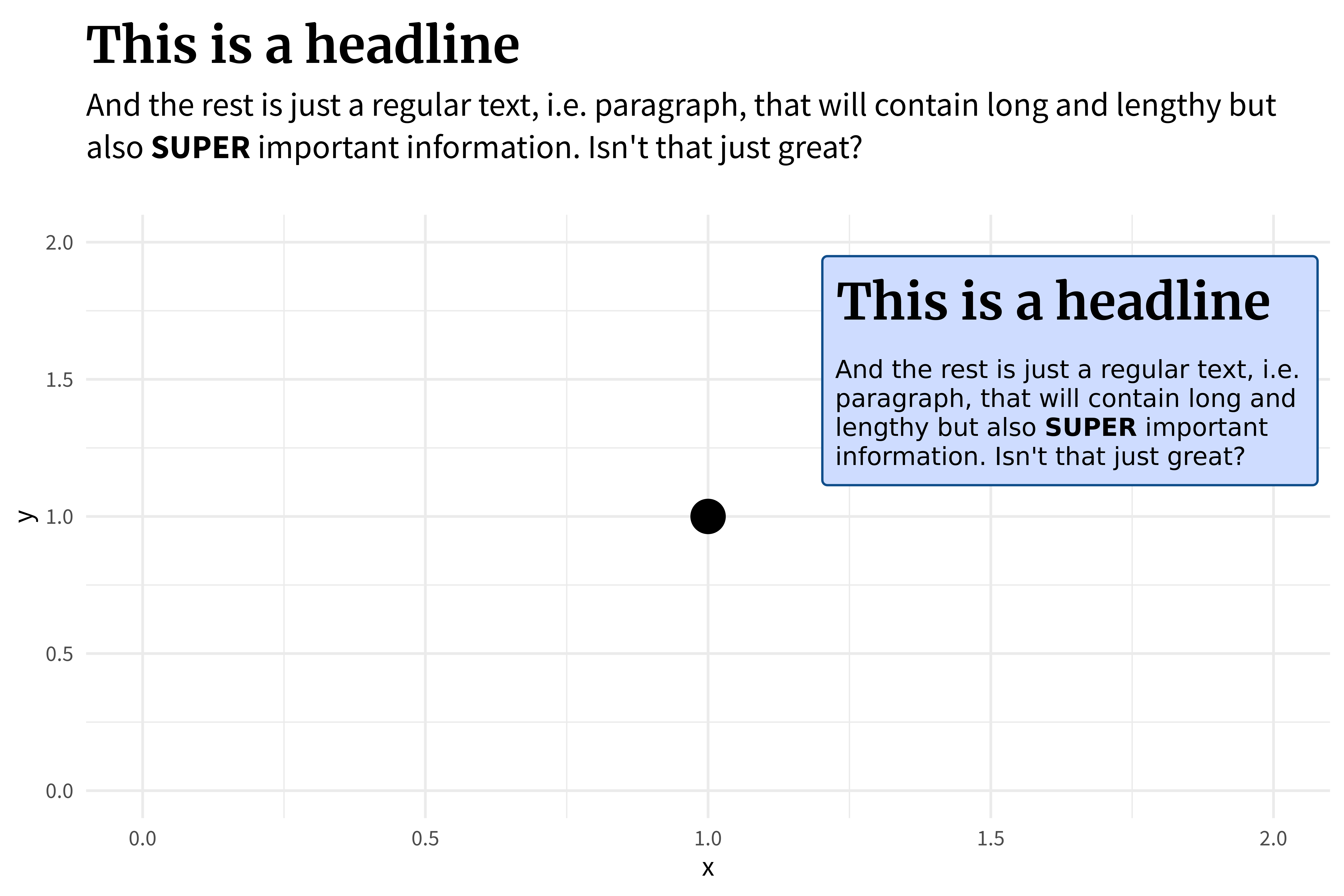
md_text <- '# This is a headline

And the rest is just a regular text, i.e. paragraph, that will contain long and lengthy but also {.red **SUPER** important information}. Isn\'t that just great?'

tibble(x = 1, y = 1) |> 
  ggplot(aes(x, y)) +
  geom_point(size = 10) +
  annotate(
    'marquee',
    x = 1.2,
    y = 1.5,
    label = md_text,
    width = 0.4,
    hjust = 0,
    fill = colorspace::lighten('dodgerblue1', 0.7),
    style = text_box_style
  ) +
  labs(title = md_text) +
  theme_minimal(
    base_size = 18, 
    base_family = 'Source Sans Pro'
  ) +
  theme(
    plot.title = element_marquee(
      width = 1,
      style = headline_style
    )
  ) +
  coord_cartesian(
    xlim = c(0, 2),
    ylim = c(0, 2)
  )

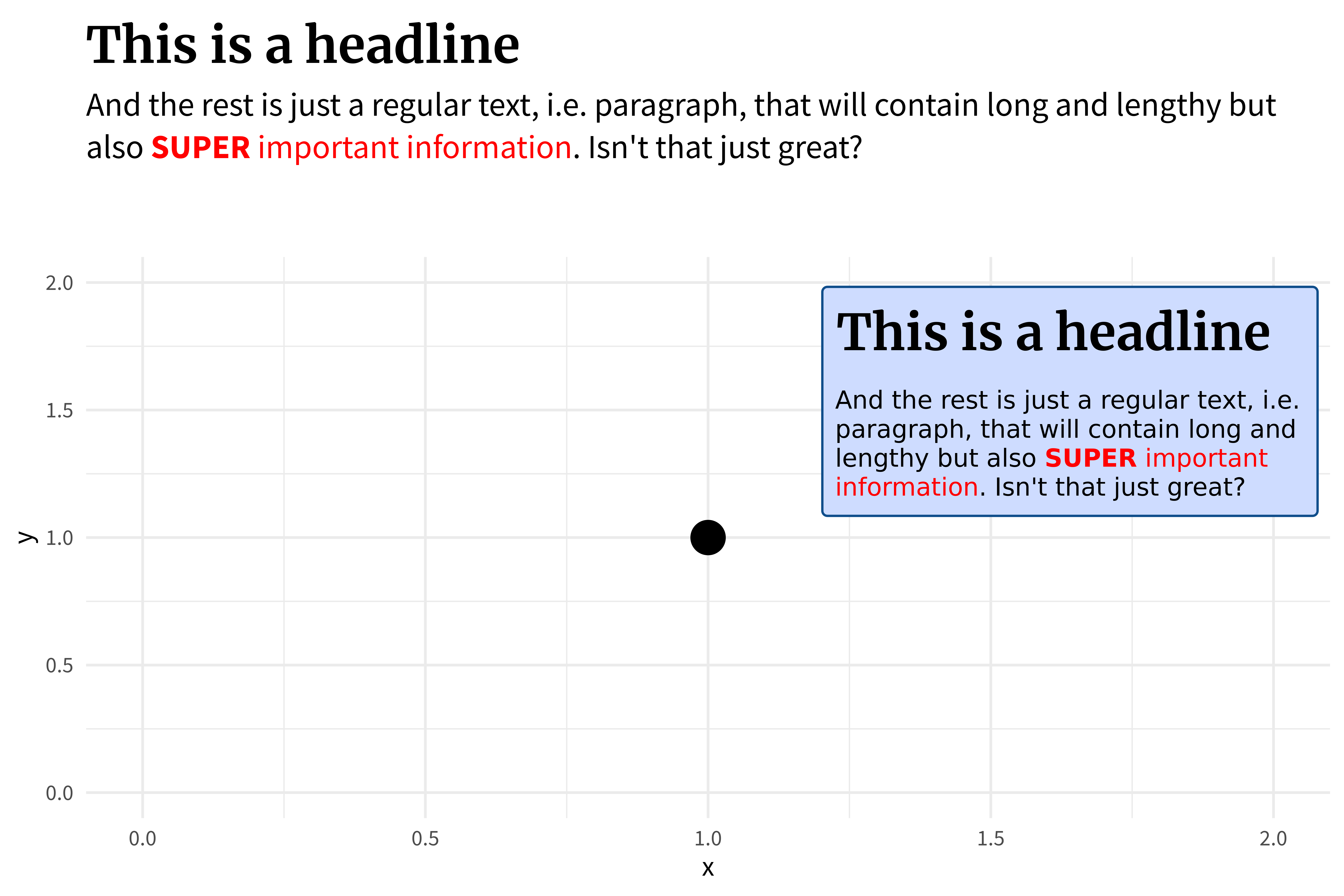
Define your own inline style

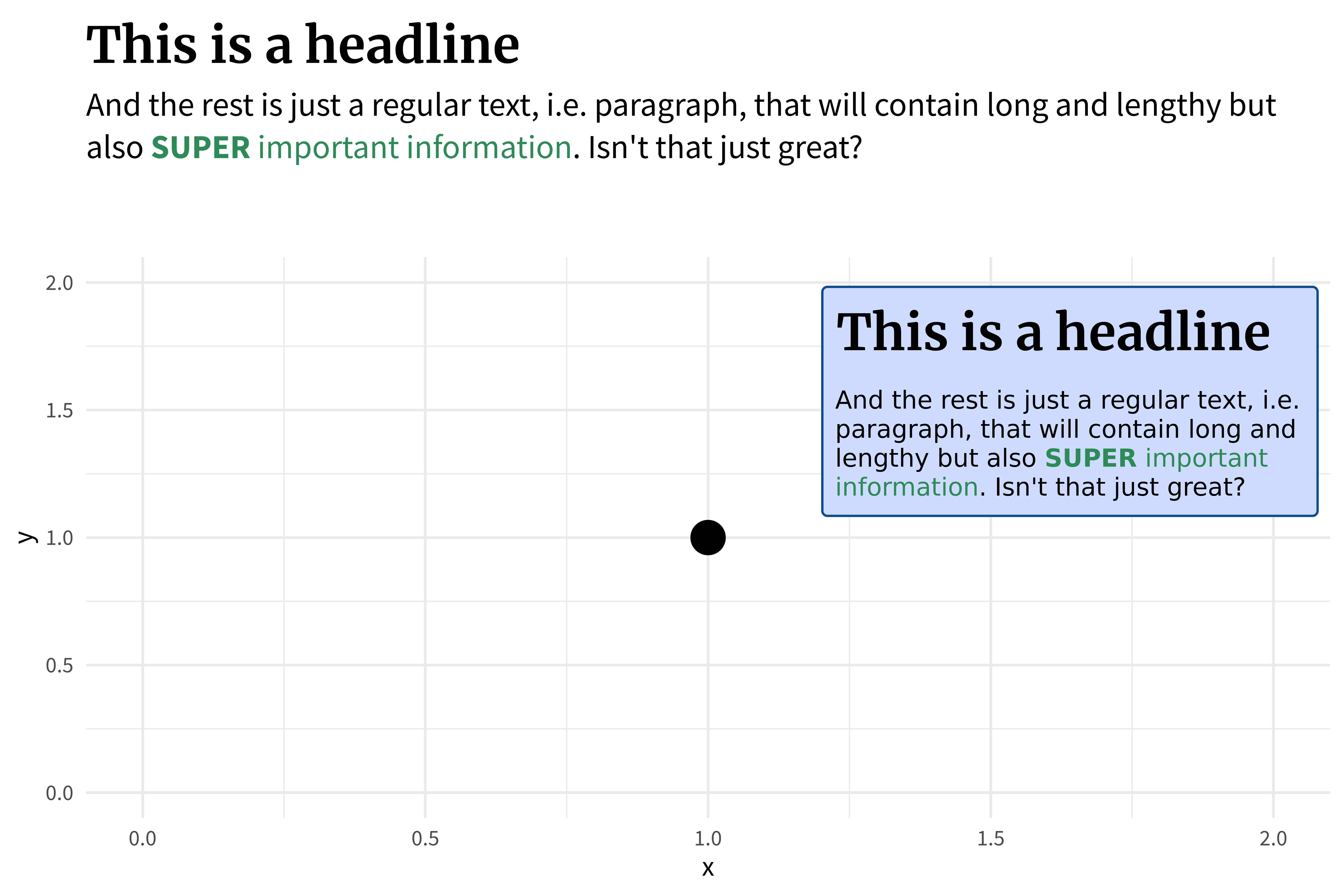
md_text <- '# This is a headline

And the rest is just a regular text, i.e. paragraph, that will contain long and lengthy but also {.my_style **SUPER** important information}. Isn\'t that just great?'

tibble(x = 1, y = 1) |> 
  ggplot(aes(x, y)) +
  geom_point(size = 10) +
  annotate(
    'marquee',
    x = 1.2,
    y = 1.5,
    label = md_text,
    width = 0.4,
    hjust = 0,
    fill = colorspace::lighten('dodgerblue1', 0.7),
    style = text_box_style |> 
      modify_style(
        'my_style',
        color = 'seagreen'
      )
  ) +
  labs(title = md_text) +
  theme_minimal(
    base_size = 18, 
    base_family = 'Source Sans Pro'
  ) +
  theme(
    plot.title = element_marquee(
      width = 1,
      style = headline_style |> 
        modify_style(
          'my_style',
          color = 'seagreen'
        )
    )
  ) +
  coord_cartesian(
    xlim = c(0, 2),
    ylim = c(0, 2)
  )